"Find the Maclaurin series expansion of the function f(x)"- this is exactly what the task in higher mathematics sounds like, which some students can do, while others cannot cope with the examples. There are several ways to expand a series in powers; here we will give a technique for expanding functions into a Maclaurin series. When developing a function in a series, you need to be good at calculating derivatives.
Example 4.7 Expand a function in powers of x
Calculations: We perform the expansion of the function according to the Maclaurin formula. First, let's expand the denominator of the function into a series ![]()
Finally, multiply the expansion by the numerator.
The first term is the value of the function at zero f (0) = 1/3.
Let's find the derivatives of the function of the first and higher orders f (x) and the value of these derivatives at the point x=0 


![]()
Next, based on the pattern of changes in the value of derivatives at 0, we write the formula for the nth derivative ![]()
So, we represent the denominator in the form of an expansion in the Maclaurin series 
We multiply by the numerator and obtain the desired expansion of the function in a series in powers of x 
As you can see, there is nothing complicated here.
All key points are based on the ability to calculate derivatives and quickly generalize the value of the higher order derivative at zero. The following examples will help you learn how to quickly arrange a function in a series.
Example 4.10 Find the Maclaurin series expansion of the function
Calculations: As you may have guessed, we will put the cosine in the numerator in a series. To do this, you can use formulas for infinitesimal quantities, or derive the expansion of the cosine through derivatives. As a result, we arrive at the following series in powers of x 
As you can see, we have a minimum of calculations and a compact representation of the series expansion.
Example 4.16 Expand a function in powers of x:
7/(12-x-x^2)
Calculations: In this kind of examples, it is necessary to expand the fraction through the sum of simple fractions.
We won’t show you how to do this now, but with the help uncertain coefficients Let's arrive at the sum of the fractions.
Next we write the denominators in exponential form 
It remains to expand the terms using the Maclaurin formula. Summing up the terms at the same powers of “x”, we compose a formula for the general term of the expansion of a function in a series 

The last part of the transition to the series at the beginning is difficult to implement, since it is difficult to combine the formulas for paired and unpaired indices (degrees), but with practice you will get better at it.
Example 4.18 Find the Maclaurin series expansion of the function
Calculations: Let's find the derivative of this function: 
Let's expand the function into a series using one of McLaren's formulas: 
We sum the series term by term based on the fact that both are absolutely identical. Having integrated the entire series term by term, we obtain the expansion of the function into a series in powers of x 
There is a transition between the last two lines of the expansion which will take a lot of your time at the beginning. Generalizing a series formula isn't easy for everyone, so don't worry about not being able to get a nice, compact formula.
Example 4.28 Find the Maclaurin series expansion of the function:
Let's write the logarithm as follows 
Using Maclaurin’s formula, we expand the logarithm function in a series in powers of x 
The final convolution is complex at first glance, but when alternating signs you will always get something similar. Input lesson on the topic of scheduling functions in a row is completed. Other equally interesting decomposition schemes will be discussed in detail in the following materials.
If the function f(x) has derivatives of all orders on a certain interval containing point a, then the Taylor formula can be applied to it:
,
Where r n– the so-called remainder term or remainder of the series, it can be estimated using the Lagrange formula:
, where the number x is between x and a.
Rules for entering functions:
If for some value X r n→0 at n→∞, then in the limit the Taylor formula becomes convergent for this value Taylor series:
,
Thus, the function f(x) can be expanded into a Taylor series at the point x under consideration if:
1) it has derivatives of all orders;
2) the constructed series converges at this point.
When a = 0 we get a series called near Maclaurin:
,
Expansion of the simplest (elementary) functions in the Maclaurin series:
Exponential functions
, R=∞
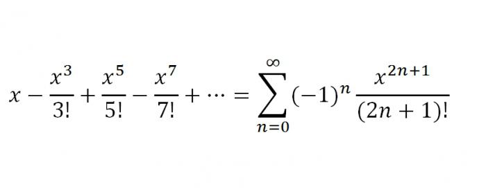
Trigonometric functions ![]() , R=∞
, R=∞ ![]() , R=∞
, R=∞
, (-π/2< x < π/2), R=π/2
The function actgx does not expand in powers of x, because ctg0=∞
Hyperbolic functions
Logarithmic functions
, -1
Binomial series
![]() .
.
Example No. 1. Expand the function into a power series f(x)= 2x.
Solution. Let us find the values of the function and its derivatives at X=0
f(x) = 2x, f( 0)
= 2 0
=1;
f"(x) = 2x ln2, f"( 0)
= 2 0
ln2= ln2;
f""(x) = 2x ln 2 2, f""( 0)
= 2 0
ln 2 2= ln 2 2;
…
f(n)(x) = 2x ln n 2, f(n)( 0)
= 2 0
ln n 2=ln n 2.
Substituting the obtained values of the derivatives into the Taylor series formula, we obtain:
The radius of convergence of this series is equal to infinity, therefore this expansion is valid for -∞<x<+∞.
Example No. 2. Write the Taylor series in powers ( X+4) for function f(x)= e x.
Solution. Finding the derivatives of the function e x and their values at the point X=-4.
f(x)= e x, f(-4)
= e -4
;
f"(x)= e x, f"(-4)
= e -4
;
f""(x)= e x, f""(-4)
= e -4
;
…
f(n)(x)= e x, f(n)( -4)
= e -4
.
Therefore, the required Taylor series of the function has the form:
This expansion is also valid for -∞<x<+∞.
Example No. 3. Expand a function f(x)=ln x in a series in powers ( X- 1),
(i.e. in the Taylor series in the vicinity of the point X=1).
Solution. Find the derivatives of this function.
f(x)=lnx , , , ,
f(1)=ln1=0, f"(1)=1, f""(1)=-1, f"""(1)=1*2,..., f (n) =(- 1) n-1 (n-1)!
Substituting these values into the formula, we obtain the desired Taylor series:
Using d'Alembert's test, you can verify that the series converges at ½x-1½<1 . Действительно,
The series converges if ½ X- 1½<1, т.е. при 0<x<2. При X=2 we obtain an alternating series that satisfies the conditions of the Leibniz criterion. When x=0 the function is not defined. Thus, the region of convergence of the Taylor series is the half-open interval (0;2].
Example No. 4. Expand the function into a power series. Example No. 5. Expand the function into a Maclaurin series. Comment
.
This method is based on the theorem on the uniqueness of the expansion of a function in a power series. The essence of this theorem is that in the neighborhood of the same point two different power series cannot be obtained that would converge to the same function, no matter how its expansion is performed. Example No. 5a. Expand the function in a Maclaurin series and indicate the region of convergence. The fraction 3/(1-3x) can be considered as the sum of an infinitely decreasing geometric progression with a denominator of 3x, if |3x|< 1. Аналогично, дробь 2/(1+2x) как сумму бесконечно убывающей геометрической прогрессии знаменателем -2x, если |-2x| < 1. В результате получим разложение в степенной ряд
Example No. 6. Expand the function into a Taylor series in the vicinity of the point x = 3. Example No. 7. Write the Taylor series in powers (x -1) of the function ln(x+2) . Example No. 8. Expand the function f(x)=sin(πx/4) into a Taylor series in the vicinity of the point x =2. Example No. 1. Calculate ln(3) to the nearest 0.01. Example No. 2. Calculate to the nearest 0.0001. Example No. 3. Calculate the integral ∫ 0 1 4 sin (x) x to within 10 -5 . Example No. 4. Calculate the integral ∫ 0 1 4 e x 2 with an accuracy of 0.001. Students of higher mathematics should know that the sum of a certain power series belonging to the interval of convergence of the series given to us turns out to be a continuous and unlimited number of times differentiated function. The question arises: is it possible to say that a given arbitrary function f(x) is the sum of a certain power series? That is, under what conditions can the function f(x) be represented by a power series? The importance of this question lies in the fact that it is possible to approximately replace the function f(x) with the sum of the first few terms of a power series, that is, a polynomial. This replacement of a function with a rather simple expression - a polynomial - is also convenient when solving certain problems, namely: when solving integrals, when calculating, etc. It has been proven that for a certain function f(x), in which it is possible to calculate derivatives up to the (n+1)th order, including the last, in the neighborhood of (α - R; x 0 + R) some point x = α, it is true that formula: This formula is named after the famous scientist Brooke Taylor. The series that is obtained from the previous one is called the Maclaurin series: The rule that makes it possible to perform an expansion in a Maclaurin series: R n (x) -> 0 at n -> infinity. If one exists, the function f(x) in it must coincide with the sum of the Maclaurin series. Let us now consider the Maclaurin series for individual functions. 1. So, the first one will be f(x) = e x. Of course, by its characteristics, such a function has derivatives of very different orders, and f (k) (x) = e x , where k equals all. Substitute x = 0. We get f (k) (0) = e 0 =1, k = 1,2... Based on the above, the series e x will look like this: 2. Maclaurin series for the function f(x) = sin x. Let us immediately clarify that the function for all unknowns will have derivatives, in addition, f "(x) = cos x = sin(x+n/2), f "" (x) = -sin x = sin(x +2*n/2)..., f (k) (x) = sin(x+k*n/2), where k is equal to any natural number. That is, after making simple calculations, we can come to the conclusion that the series for f(x) = sin x will look like this: 3. Now let's try to consider the function f(x) = cos x. For all unknowns it has derivatives of arbitrary order, and |f (k) (x)| = |cos(x+k*n/2)|<=1, k=1,2... Снова-таки, произведя определенные расчеты, получим, что ряд для f(х) = cos х будет выглядеть так: So, we have listed the most important functions that can be expanded in a Maclaurin series, but they are supplemented by Taylor series for some functions. Now we will list them. It is also worth noting that Taylor and Maclaurin series are an important part of practical work on solving series in higher mathematics. So, Taylor series. 1. The first will be the series for the function f(x) = ln(1+x). As in the previous examples, for the given f(x) = ln(1+x) we can add the series using the general form of the Maclaurin series. however, for this function the Maclaurin series can be obtained much more simply. Having integrated a certain geometric series, we obtain a series for f(x) = ln(1+x) of such a sample: 2. And the second, which will be final in our article, will be the series for f(x) = arctan x. For x belonging to the interval [-1;1] the expansion is valid: That's all. This article examined the most used Taylor and Maclaurin series in higher mathematics, in particular in economics and technical universities. If the function f(x) has on some interval containing the point A, derivatives of all orders, then the Taylor formula can be applied to it: Where r n– the so-called remainder term or remainder of the series, it can be estimated using the Lagrange formula: If for some value x r n®0 at n®¥, then in the limit the Taylor formula turns into a convergent formula for this value Taylor series: So the function f(x) can be expanded into a Taylor series at the point in question X, If: 1) it has derivatives of all orders; 2) the constructed series converges at this point. At A=0 we get a series called near Maclaurin: Example 1
f(x)= 2x. Solution. Let us find the values of the function and its derivatives at X=0 f(x) = 2x, f( 0)
= 2 0
=1; f¢(x) = 2x ln2, f¢( 0)
= 2 0
ln2= ln2; f¢¢(x) = 2x ln 2 2, f¢¢( 0)
= 2 0
ln 2 2= ln 2 2; f(n)(x) = 2x ln n 2, f(n)( 0)
= 2 0
ln n 2=ln n 2. Substituting the obtained values of the derivatives into the Taylor series formula, we obtain: The radius of convergence of this series is equal to infinity, therefore this expansion is valid for -¥<x<+¥. Example 2
X+4) for function f(x)= e x. Solution. Finding the derivatives of the function e x and their values at the point X=-4. f(x)= e x, f(-4)
= e -4
; f¢(x)= e x, f¢(-4)
= e -4
; f¢¢(x)= e x, f¢¢(-4)
= e -4
; f(n)(x)= e x, f(n)( -4)
= e -4
. Therefore, the required Taylor series of the function has the form: This expansion is also valid for -¥<x<+¥. Example 3
. Expand a function f(x)=ln x in a series in powers ( X- 1), (i.e. in the Taylor series in the vicinity of the point X=1). Solution. Find the derivatives of this function. Substituting these values into the formula, we obtain the desired Taylor series: Using d'Alembert's test, you can verify that the series converges when ½ X- 1½<1. Действительно, The series converges if ½ X- 1½<1, т.е. при 0<x<2. При X=2 we obtain an alternating series that satisfies the conditions of the Leibniz criterion. At X=0 function is not defined. Thus, the region of convergence of the Taylor series is the half-open interval (0;2]. Let us present the expansions obtained in this way into the Maclaurin series (i.e. in the vicinity of the point X=0) for some elementary functions: (2) (3) ( the last decomposition is called binomial series) Example 4
. Expand the function into a power series Solution. In expansion (1) we replace X on - X 2, we get: Example 5
. Expand the function in a Maclaurin series Solution. We have Using formula (4), we can write: substituting instead X into the formula -X, we get: From here we find: Opening the brackets, rearranging the terms of the series and bringing similar terms, we get This series converges in the interval (-1;1), since it is obtained from two series, each of which converges in this interval. Comment
. Formulas (1)-(5) can also be used to expand the corresponding functions into a Taylor series, i.e. for expanding functions in positive integer powers ( Ha). To do this, it is necessary to perform such identical transformations on a given function in order to obtain one of the functions (1)-(5), in which instead X costs k( Ha) m , where k is a constant number, m is a positive integer. It is often convenient to make a change of variable t=Ha and expand the resulting function with respect to t in the Maclaurin series. This method illustrates the theorem on the uniqueness of a power series expansion of a function. The essence of this theorem is that in the neighborhood of the same point two different power series cannot be obtained that would converge to the same function, no matter how its expansion is performed. Example 6
. Expand the function in a Taylor series in a neighborhood of a point X=3. Solution. This problem can be solved, as before, using the definition of the Taylor series, for which we need to find the derivatives of the function and their values at X=3. However, it will be easier to use the existing expansion (5): The resulting series converges at Example 7
. Write the Taylor series in powers ( X-1) functions Solution. The series converges at
Solution. In expansion (1) we replace x with -x 2, we get:
, -∞
Solution. We have
Using formula (4), we can write:
substituting –x instead of x in the formula, we get:
From here we find: ln(1+x)-ln(1-x) = -
Opening the brackets, rearranging the terms of the series and bringing similar terms, we get
. This series converges in the interval (-1;1), since it is obtained from two series, each of which converges in this interval.
Formulas (1)-(5) can also be used to expand the corresponding functions into a Taylor series, i.e. for expanding functions in positive integer powers ( Ha). To do this, it is necessary to perform such identical transformations on a given function in order to obtain one of the functions (1)-(5), in which instead X costs k( Ha) m , where k is a constant number, m is a positive integer. It is often convenient to make a change of variable t=Ha and expand the resulting function with respect to t in the Maclaurin series.
Solution. First we find 1-x-6x 2 =(1-3x)(1+2x) , .
to elementary:
with convergence region |x|< 1/3.
Solution. This problem can be solved, as before, using the definition of the Taylor series, for which we need to find the derivatives of the function and their values at X=3. However, it will be easier to use the existing expansion (5):
=
The resulting series converges at or –3
Solution.
The series converges at , or -2< x < 5.
Solution. Let's make the replacement t=x-2:
Using expansion (3), in which we substitute π / 4 t in place of x, we obtain:
The resulting series converges to the given function at -∞< π / 4 t<+∞, т.е. при (-∞
, (-∞Approximate calculations using power series
Power series are widely used in approximate calculations. With their help, you can calculate the values of roots, trigonometric functions, logarithms of numbers, and definite integrals with a given accuracy. Series are also used when integrating differential equations.
Consider the expansion of a function in a power series:
In order to calculate the approximate value of a function at a given point X, belonging to the region of convergence of the indicated series, the first ones are left in its expansion n members ( n– a finite number), and the remaining terms are discarded:
To estimate the error of the obtained approximate value, it is necessary to estimate the discarded remainder rn (x) . To do this, use the following techniques:
Solution. Let's use the expansion where x=1/2 (see example 5 in the previous topic):
Let's check whether we can discard the remainder after the first three terms of the expansion; to do this, we will evaluate it using the sum of an infinitely decreasing geometric progression:
So we can discard this remainder and get
Solution. Let's use the binomial series. Since 5 3 is the cube of an integer closest to 130, it is advisable to represent the number 130 as 130 = 5 3 +5. 
since already the fourth term of the resulting alternating series satisfying the Leibniz criterion is less than the required accuracy:
, so it and the terms following it can be discarded.
Many practically necessary definite or improper integrals cannot be calculated using the Newton-Leibniz formula, because its application is associated with finding the antiderivative, which often does not have an expression in elementary functions. It also happens that finding an antiderivative is possible, but it is unnecessarily labor-intensive. However, if the integrand function is expanded into a power series, and the limits of integration belong to the interval of convergence of this series, then an approximate calculation of the integral with a predetermined accuracy is possible.
Solution. The corresponding indefinite integral cannot be expressed in elementary functions, i.e. represents a “non-permanent integral”. The Newton-Leibniz formula cannot be applied here. Let's calculate the integral approximately.
Dividing term by term the series for sin x on x, we get: 
Integrating this series term by term (this is possible, since the limits of integration belong to the interval of convergence of this series), we obtain:
Since the resulting series satisfies Leibniz’s conditions and it is enough to take the sum of the first two terms to obtain the desired value with a given accuracy.
Thus, we find  .
.
Solution.

![]() . Let's check whether we can discard the remainder after the second term of the resulting series.
. Let's check whether we can discard the remainder after the second term of the resulting series.
0.0001<0.001. Следовательно,  .
.


 , where the number x is between X And A.
![]()
![]()
![]()
![]()
![]()

![]() ,
,
![]() ,
,![]()
![]()


![]() or –3<x- 3<3, 0<x< 6 и является искомым рядом Тейлора для данной функции.
or –3<x- 3<3, 0<x< 6 и является искомым рядом Тейлора для данной функции.![]() .
.![]() , or 2< x£5.
, or 2< x£5.


