You can also search not for the best point in the direction of the gradient, but for some one better than the current one.
The easiest to implement of all local optimization methods. Has quite weak conditions convergence, but the rate of convergence is quite low (linear). The gradient method step is often used as part of other optimization methods, such as the Fletcher–Reeves method.
Description [ | ]
Improvements[ | ]
The gradient descent method turns out to be very slow when moving along a ravine, and with an increase in the number of variables objective function This behavior of the method becomes typical. To combat this phenomenon, it is used, the essence of which is very simple. Having made two steps of gradient descent and obtained three points, the third step should be taken in the direction of the vector connecting the first and third points, along the bottom of the ravine.
For functions close to quadratic, the conjugate gradient method is effective.
Application in artificial neural networks[ | ]
The gradient descent method, with some modification, is widely used for perceptron training and is known in the theory of artificial neural networks as the backpropagation method. When training a perceptron-type neural network, it is necessary to change the weighting coefficients of the network so as to minimize average error at the output of the neural network when a sequence of training input data is supplied to the input. Formally, in order to take just one step using the gradient descent method (make just one change in the network parameters), it is necessary to sequentially submit absolutely the entire set of training data to the network input, calculate the error for each object of the training data and calculate the necessary correction of the network coefficients (but not do this correction), and after submitting all the data, calculate the amount in the adjustment of each network coefficient (sum of gradients) and correct the coefficients “one step”. Obviously, with a large set of training data, the algorithm will work extremely slowly, so in practice, network coefficients are often adjusted after each training element, where the gradient value is approximated by the gradient of the cost function, calculated on only one training element. This method is called stochastic gradient descent or operational gradient descent . Stochastic gradient descent is a form of stochastic approximation. The theory of stochastic approximations provides conditions for the convergence of the stochastic gradient descent method.
Links [ | ]
- J. Mathews. Module for Steepest Descent or Gradient Method. (unavailable link)
Literature [ | ]
- Akulich I. L. Mathematical programming in examples and problems. - M.: Higher School, 1986. - P. 298-310.
- Gill F., Murray W., Wright M. Practical optimization = Practical Optimization. - M.: Mir, 1985.
- Korshunov Yu. M., Korshunov Yu. M. Mathematical foundations of cybernetics. - M.: Energoatomizdat, 1972.
- Maksimov Yu. A., Fillipovskaya E. A. Algorithms for solving nonlinear programming problems. - M.: MEPhI, 1982.
- Maksimov Yu. A. Algorithms for linear and discrete programming. - M.: MEPhI, 1980.
- Korn G., Korn T. Handbook of mathematics for scientists and engineers. - M.: Nauka, 1970. - P. 575-576.
- S. Yu. Gorodetsky, V. A. Grishagin. Nonlinear programming and multiextremal optimization. - Nizhny Novgorod: Nizhny Novgorod University Publishing House, 2007. - pp. 357-363.
The steepest descent method is a gradient method with a variable step. At each iteration, the step size k is selected from the condition of the minimum of the function f(x) in the direction of descent, i.e.
This condition means that movement along the antigradient occurs as long as the value of the function f (x) decreases. From a mathematical point of view, at each iteration it is necessary to solve the problem of one-dimensional minimization by function
()=f (x (k) -f (x (k)))
Let's use the golden ratio method for this.
The algorithm of the steepest descent method is as follows.
The coordinates of the starting point x (0) are specified.
At point x (k) , k = 0, 1, 2, ..., the gradient value f (x (k)) is calculated.
The step size k is determined by one-dimensional minimization using the function
()=f (x (k) -f (x (k))).
The coordinates of the point x (k) are determined:
x i (k+1) = x i (k) - k f i (x (k)), i=1, …, n.
The condition for stopping the iterative process is checked:
||f (x (k +1))|| .
If it is fulfilled, then the calculations stop. Otherwise, we proceed to step 1. The geometric interpretation of the steepest descent method is presented in Fig. 1.

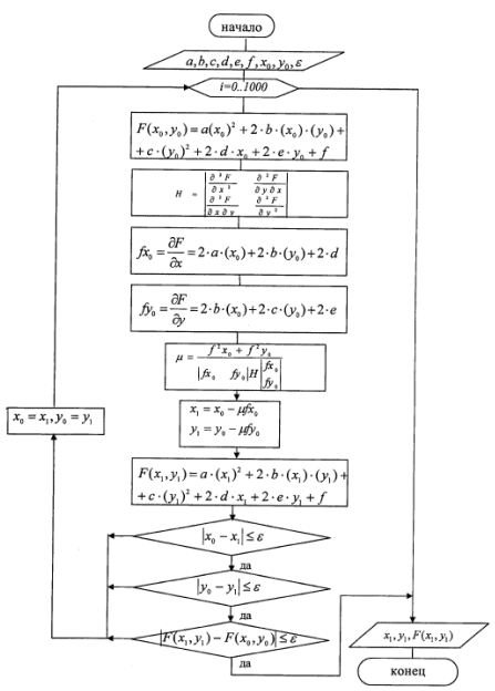
Rice. 2.1. Block diagram of the steepest descent method.
Implementation of the method in the program:
Method of steepest descent.

Rice. 2.2. Implementation of the steepest descent method.
Conclusion: In our case, the method converged in 7 iterations. Point A7 (0.6641; -1.3313) is an extremum point. Method of conjugate directions. For quadratic functions, you can create a gradient method in which the convergence time will be finite and equal to the number of variables n.
Let us call a certain direction and conjugate with respect to some positive definite Hess matrix H if:
Then i.e. So for unit H, the conjugate direction means their perpendicular. In the general case, H is non-trivial. IN general case conjugacy is the application of the Hess matrix to a vector - it means rotating this vector by some angle, stretching or compressing it.

And now the vector is orthogonal, i.e. conjugacy is not the orthogonality of the vector, but the orthogonality of the rotated vector.e.i.


Rice. 2.3. Block diagram of the conjugate directions method.
Implementation of the method in the program: Method of conjugate directions.

Rice. 2.4. Implementation of the conjugate directions method.

Rice. 2.5. Graph of the conjugate directions method.
Conclusion: Point A3 (0.6666; -1.3333) was found in 3 iterations and is an extremum point.
3. Analysis of methods for determining the minimum and maximum value of a function in the presence of restrictions
Let us recall that common task conditional optimization looks like this
f(x) ® min, x О W,
where W is a proper subset of R m. A subclass of problems with equality-type constraints is distinguished by the fact that the set is defined by constraints of the form
f i (x) = 0, where f i: R m ®R (i = 1, …, k).
Thus,W = (x О R m: f i (x) = 0, i = 1, …, k).
It will be convenient for us to write index "0" for the function f. Thus, the optimization problem with equality type constraints is written as
f 0 (x) ® min, (3.1)
f i (x) = 0, i = 1, …, k. (3.2)
If we now denote by f a function on R m with values in R k, the coordinate notation of which has the form f(x) = (f 1 (x), ..., f k (x)), then (3.1)–(3.2) we can also write it in the form
f 0 (x) ® min, f(x) = Q.
Geometrically, a problem with equality type constraints is a problem of finding the lowest point of the graph of a function f 0 over the manifold (see Fig. 3.1).

Points that satisfy all the constraints (i.e., points in the set ) are usually called admissible. An admissible point x* is called a conditional minimum of the function f 0 under the constraints f i (x) = 0, i = 1, ..., k (or a solution to problem (3.1)–(3.2)), if for all admissible points x f 0 (x *) f 0 (x). (3.3)
If (3.3) is satisfied only for admissible x lying in some neighborhood V x * of point x*, then we speak of a local conditional minimum. The concepts of conditional strict local and global minima are defined in a natural way.
In this version of the gradient method, the minimizing sequence (X k) is also constructed according to rule (2.22). However, the step size a k is found as a result of solving the auxiliary one-dimensional minimization problem
min(j k (a) | a>0 ), (2.27)
where j k (a)=f(X k - a· (X k)). Thus, at each iteration in the direction of the antigradient ![]() an exhaustive descent is performed. To solve problem (2.27), you can use one of the one-dimensional search methods described in Section 1, for example, the bitwise search method or the golden section method.
an exhaustive descent is performed. To solve problem (2.27), you can use one of the one-dimensional search methods described in Section 1, for example, the bitwise search method or the golden section method.
Let us describe the algorithm of the steepest descent method.
Step 0. Set the accuracy parameter e>0, select X 0 ОE n , set k=0.
Step 1. Find (X k) and check the condition for achieving the specified accuracy || (x k) ||£ e. If it is satisfied, then go to step 3, otherwise - to step 2.
Step 2. Solve problem (2.27), i.e. find a k. Find the next point, put k=k+1 and go to step 1.
Step 3 Complete the calculations by putting X * = X k, f * = f(X k).
Minimize function
f(x)=x 1 2 +4x 2 2 -6x 1 -8x 2 +13; (2.28)
Let's solve the problem first classic method. Let us write down a system of equations representing the necessary conditions unconditional extremum

Having solved it, we obtain a stationary point X*=(3;1). Next, let's check the execution sufficient condition, for which we find the matrix of second derivatives
Since, according to the Sylvester criterion, this matrix is positive definite for ", then the found point X* is the minimum point of the function f(X). The minimum value f *=f(X*)=0. This is the exact solution to problem (11).
Let's perform one iteration of the method gradient descent for (2.28). Let's choose the starting point X 0 =(1;0), set the initial step a=1 and the parameter l=0.5. Let's calculate f(X 0)=8.
Let's find the gradient of the function f(X) at point X 0
(X 0)= = (2.29)
Let's define a new point X=X 0 -a· (X 0) by calculating its coordinates
x 1 = 
x 2 =  (2.30)
Let's calculate f(X)= f(X 0 -a· (X 0))=200. Since f(X)>f(X 0), we split the step, assuming a=a·l=1·0.5=0.5. We calculate again using formulas (2.30) x 1 =1+4a=3; x 2 =8a=4 and find the value f(X)=39. Since f(X)>f(X 0) again, we further reduce the step size, setting a=a·l=0.5·0.5=0.25. We calculate a new point with coordinates x 1 =1+4·0.25=2; x 2 =8·0.25=2 and the value of the function at this point f(X)=5. Since the condition for decreasing f(X) Let's perform one iteration using the method steepest descent for (2.28) with the same initial point X 0 =(1;0). Using the already found gradient (2.29), we find X= X 0 -a· (X 0) and construct the function j 0 (a)=f(X 0 -a· (X 0))=(4a-2) 2 +4(8a-1) 2. By minimizing it using the necessary condition j 0 ¢(a)=8·(4a - 2)+64·(8a - 1)=0 we find the optimal value of the step size a 0 =5/34. Determining the point of the minimizing sequence X 1 = X 0 -a 0 · (X 0) The gradient of the differentiable function f(x) at the point X called n-dimensional vector f(x)
, whose components are partial derivatives of the function f(x), calculated at the point X, i.e. f"(x ) = (df(x)/dh 1 , …, df(x)/dx n) T . This vector is perpendicular to the plane through the point X, and tangent to the level surface of the function f(x), passing through a point X.At each point of such a surface the function f(x) takes the same value. Equating the function to various constant values C 0 , C 1 , ..., we obtain a series of surfaces characterizing its topology (Fig. 2.8). The gradient vector is directed in the direction of the fastest increase in the function at a given point. Vector opposite to gradient (-f’(x))
, called anti-gradient and is directed towards the fastest decrease of the function. At the minimum point, the gradient of the function is zero. First-order methods, also called gradient and minimization methods, are based on the properties of gradients. Using these methods in the general case allows you to determine the local minimum point of a function. Obviously, if there is no additional information, then from the starting point X it's wise to go to the point X, lying in the direction of the antigradient - the fastest decrease of the function. Choosing as the direction of descent R[k] anti-gradient - f'(x[k] )
at the point X[k], we obtain an iterative process of the form X[ k+ 1] = x[k]-a k f"(x[k] )
,
and k > 0; k=0, 1, 2, ... In coordinate form, this process is written as follows: x i [ k+1]=x i[k] - a kf(x[k] )
/x i i = 1, ..., n; k= 0, 1, 2,... As a criterion for stopping the iterative process, either the fulfillment of the condition of small increment of the argument || x[k+l] -x[k] || <= e
,
либо выполнение условия малости градиента || f'(x[k+l] )
|| <= g
, Here e and g are given small quantities. A combined criterion is also possible, consisting in the simultaneous fulfillment of the specified conditions. Gradient methods differ from each other in the way they choose the step size and k. In the method with a constant step, a certain constant step value is selected for all iterations. Quite a small step and k will ensure that the function decreases, i.e., the inequality f(x[ k+1])
= f(x[k] – a k f’(x[k] ))
< f(x[k] )
. However, this may lead to the need to carry out an unacceptably large number of iterations to reach the minimum point. On the other hand, a step that is too large can cause an unexpected increase in the function or lead to oscillations around the minimum point (cycling). Due to the difficulty of obtaining the necessary information to select the step size, methods with constant steps are rarely used in practice. Gradient ones are more economical in terms of the number of iterations and reliability variable step methods, when, depending on the results of calculations, the step size changes in some way. Let us consider the variants of such methods used in practice. When using the steepest descent method at each iteration, the step size and k is selected from the minimum condition of the function f(x) in the direction of descent, i.e. This condition means that movement along the antigradient occurs as long as the value of the function f(x) decreases. From a mathematical point of view, at each iteration it is necessary to solve the problem of one-dimensional minimization according to A functions The algorithm of the steepest descent method is as follows. 1. Set the coordinates of the starting point X.
2. At the point X[k],
k = 0, 1, 2, ... calculates the gradient value f'(x[k])
. 3. The step size is determined a k, by one-dimensional minimization over A functions j (a) = f(x[k]-af"(x[k])).
4. The coordinates of the point are determined X[k+ 1]: x i [ k+ 1]= x i[k]– a k f’ i (x[k]), i = 1,..., p. 5. The conditions for stopping the steration process are checked. If they are fulfilled, then the calculations stop. Otherwise, go to step 1. In the method under consideration, the direction of movement from the point X[k] touches the level line at the point x[k+ 1] (Fig. 2.9). The descent trajectory is zigzag, with adjacent zigzag links orthogonal to each other. Indeed, a step a k is chosen by minimizing by A functions? (a) = f(x[k] -af"(x[k]))
. Necessary condition for the minimum of a function d j (a)/da = 0. Having calculated the derivative of a complex function, we obtain the condition for the orthogonality of the vectors of descent directions at neighboring points: dj (a)/da = -f’(x[k+ 1]f'(x[k])
= 0.
Gradient methods converge to a minimum at high speed (geometric progression speed) for smooth convex functions. Such functions have the greatest M and least m eigenvalues of the matrix of second derivatives (Hessian matrix) differ little from each other, i.e. the matrix N(x) well conditioned. Recall that the eigenvalues l i, i
=1, …, n, the matrices are the roots of the characteristic equation However, in practice, as a rule, the functions being minimized have ill-conditioned matrices of second derivatives (t/m<<
1). The values of such functions along some directions change much faster (sometimes by several orders of magnitude) than in other directions. Their level surfaces in the simplest case are strongly elongated (Fig. 2.10), and in more complex cases they bend and look like ravines. Functions with such properties are called gully. The direction of the antigradient of these functions (see Fig. 2.10) deviates significantly from the direction to the minimum point, which leads to a slowdown in the speed of convergence. The convergence rate of gradient methods also depends significantly on the accuracy of gradient calculations. Loss of accuracy, which usually occurs in the vicinity of minimum points or in a gully situation, can generally disrupt the convergence of the gradient descent process. Due to the above reasons, gradient methods are often used in combination with other, more effective methods at the initial stage of solving a problem. In this case, the point X is far from the minimum point, and steps in the direction of the antigradient make it possible to achieve a significant decrease in the function. The gradient methods discussed above find the minimum point of a function in the general case only in an infinite number of iterations. The conjugate gradient method generates search directions that are more consistent with the geometry of the function being minimized. This significantly increases the speed of their convergence and allows, for example, to minimize the quadratic function f(x) = (x, Hx) + (b, x) + a with a symmetric positive definite matrix N in a finite number of steps P, equal to the number of function variables. Any smooth function in the vicinity of the minimum point can be well approximated by a quadratic function, therefore conjugate gradient methods are successfully used to minimize non-quadratic functions. In this case, they cease to be finite and become iterative. By definition, two n-dimensional vector X And at called conjugated relative to the matrix H(or H-conjugate), if the scalar product (x, Well) = 0. Here N - symmetric positive definite matrix of size P X P. One of the most significant problems in conjugate gradient methods is the problem of efficiently constructing directions. The Fletcher-Reeves method solves this problem by transforming the antigradient at each step -f(x[k])
in the direction p[k],
H-conjugate with previously found directions R, R, ..., R[k-1]. Let us first consider this method in relation to the minimization problem quadratic function. Directions R[k] is calculated using the formulas: p[ k] = -f'(x[k])
+b k-1 p[k-l], k>= 1; p = - f’(x)
. b values k-1 are chosen so that the directions p[k], R[k-1] were H-conjugate :
(p[k], HP[k- 1])= 0.
As a result, for the quadratic function the iterative minimization process has the form x[ k+l] =x[k]+a k p[k], Where R[k] -
direction of descent to k- m step; and k - step size. The latter is selected from the minimum condition of the function f(x) By A in the direction of movement, i.e. as a result of solving the one-dimensional minimization problem: f(x[ k] + a k r[k])
= f(x[k] + ar [k])
. For a quadratic function The algorithm of the Fletcher-Reeves conjugate gradient method is as follows. 1. At the point X calculated p = -f'(x)
. 2. On k- m step, using the above formulas, the step is determined A k .
and period X[k+ 1]. 3. Values are calculated f(x[k+1])
And f'(x[k+1])
. 4. If f'(x)
= 0, then point X[k+1] is the minimum point of the function f(x). Otherwise, a new direction is determined p[k+l] from the relation and the transition to the next iteration is carried out. This procedure will find the minimum of a quadratic function in no more than P steps. When minimizing non-quadratic functions, the Fletcher-Reeves method becomes iterative from finite. In this case, after (p+ 1)th iteration of procedure 1-4 are repeated cyclically with replacement X on X[P+1] , and calculations end at , where is a given number. In this case, the following modification of the method is used: x[ k+l] = x[k]+a k p[k],
p[ k] = -f’(x[k])+
b k- 1 p[k-l], k>= 1; p = -f’( x); f(x[ k] + a k p[k])
= f(x[k] +ap[k];
Here I- many indexes: I= (0, n, 2 p, salary, ...), i.e. the method is updated every P steps. Geometric meaning The conjugate gradient method is as follows (Fig. 2.11). From a given starting point X descent is carried out in the direction R = -f"(x). At the point X the gradient vector is determined f"(x). Because the X is the minimum point of the function in the direction R,
That f'(x)
orthogonal to vector R. Then the vector is found R , H-conjugate to R. Next, we find the minimum of the function along the direction R etc. Conjugate direction methods are among the most effective for solving minimization problems. However, it should be noted that they are sensitive to errors that occur during the counting process. With a large number of variables, the error can increase so much that the process will have to be repeated even for a quadratic function, i.e. the process for it does not always fit into P steps. The steepest descent method (in English literature “method of steepest descent”) is an iterative numerical method (first order) for solving optimization problems, which allows you to determine the extremum (minimum or maximum) of the objective function: In accordance with the method under consideration, the extremum (maximum or minimum) of the objective function is determined in the direction of the fastest increase (decrease) of the function, i.e. in the direction of the gradient (anti-gradient) of the function. Gradient function at a point where i, j,…, n are unit vectors parallel to the coordinate axes. Gradient at base point The steepest descent method is further development gradient descent method. In general, the process of finding the extremum of a function is an iterative procedure, which is written as follows: where the "+" sign is used to find the maximum of a function, and the "-" sign is used to find the minimum of a function; Unit direction vector, which is determined by the formula: A constant that determines the step size and is the same for all i-th directions. The step size is selected from the condition of the minimum of the objective function f(x) in the direction of movement, i.e., as a result of solving the one-dimensional optimization problem in the direction of the gradient or antigradient: In other words, the step size is determined by solving this equation: Thus, the calculation step is chosen such that the movement is carried out until the function improves, thus reaching an extremum at some point. At this point, the search direction is determined again (using the gradient) and a new optimum point of the objective function is sought, etc. Thus, in this method, the search occurs in larger steps, and the gradient of the function is calculated at a smaller number of points. In the case of a function of two variables this method has the following geometric interpretation: the direction of movement from a point touches the level line at point . The descent trajectory is zigzag, with adjacent zigzag links orthogonal to each other. The condition for the orthogonality of the vectors of descent directions at neighboring points is written by the following expression: The trajectory of movement to the extremum point using the steepest descent method, shown on the graph of the line of equal level of the function f(x) The search for an optimal solution ends when at the iterative calculation step (several criteria): The search trajectory remains in a small neighborhood of the current search point: The increment of the objective function does not change: The gradient of the objective function at the local minimum point becomes zero: It should be noted that the gradient descent method turns out to be very slow when moving along a ravine, and as the number of variables in the objective function increases, this behavior of the method becomes typical. The ravine is a depression, the level lines of which approximately have the shape of ellipses with semi-axes differing many times over. In the presence of a ravine, the descent trajectory takes the form of a zigzag line with a small step, as a result of which the resulting speed of descent to a minimum is greatly slowed down. This is explained by the fact that the direction of the antigradient of these functions deviates significantly from the direction to the minimum point, which leads to an additional delay in the calculation. As a result, the algorithm loses computational efficiency. Gully function The gradient method, along with its many modifications, is widespread and effective method searching for the optimum of the objects under study. The disadvantage of gradient search (as well as the methods discussed above) is that when using it, only the local extremum of the function can be detected. To find others local extremes it is necessary to search from other starting points. Also the speed of convergence gradient methods also depends significantly on the accuracy of the gradient calculations. Loss of accuracy, which usually occurs in the vicinity of minimum points or in a gully situation, can generally disrupt the convergence of the gradient descent process. Calculation method Step 1: Definition of analytical expressions (in symbolic form) for calculating the gradient of a function Step 2: Set the initial approximation Step 3: The need to restart the algorithmic procedure to reset the last search direction is determined. As a result of the restart, the search is carried out again in the direction of the fastest descent.
 .
.
f(x[k]–a k f’(x[k]))
= f(x[k] – af"(x[k]))
.
j (a) = f(x[k]-af"(x[k]))
.


![]() ,
,![]()
 .
.
![]() are the values of the function argument (controlled parameters) on the real domain.
are the values of the function argument (controlled parameters) on the real domain.![]() is a vector whose projections onto the coordinate axes are the partial derivatives of the function with respect to the coordinates:
is a vector whose projections onto the coordinate axes are the partial derivatives of the function with respect to the coordinates:![]() is strictly orthogonal to the surface, and its direction shows the direction of the fastest increase in the function, and the opposite direction (antigradient), respectively, shows the direction of the fastest decrease of the function.
is strictly orthogonal to the surface, and its direction shows the direction of the fastest increase in the function, and the opposite direction (antigradient), respectively, shows the direction of the fastest decrease of the function.

![]() - the gradient module determines the rate of increase or decrease of the function in the direction of the gradient or anti-gradient:
- the gradient module determines the rate of increase or decrease of the function in the direction of the gradient or anti-gradient:
![]()
![]()

![]()


