There are two types of estimates in statistics: point and interval. Point estimate represents a separate sample statistic that is used to estimate a parameter population. For example, the sample mean is a point estimate mathematical expectation population, and sample variance S 2- point estimate of population variance σ 2. it has been shown that the sample mean is an unbiased estimate of the mathematical expectation of the population. A sample mean is called unbiased because the average of all sample means (with the same sample size) n) is equal to the mathematical expectation of the general population.

In order for the sample variance S 2 became an unbiased estimate of the population variance σ 2, the denominator of the sample variance should be set equal to n – 1 , but not n. In other words, the population variance is the average of all possible sample variances.

When estimating population parameters, it should be kept in mind that sample statistics such as , depend on specific samples. To take this fact into account, to obtain interval estimation mathematical expectation of the general population, analyze the distribution of sample means (for more details, see). The constructed interval is characterized by a certain confidence level, which represents the probability that the true population parameter is estimated correctly. Similar confidence intervals can be used to estimate the proportion of a characteristic R and the main distributed mass of the population.

Download the note in or format, examples in format

Constructing a confidence interval for the mathematical expectation of the population with a known standard deviation

Constructing a confidence interval for the share of a characteristic in the population

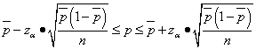
This section extends the concept of confidence interval to categorical data. This allows us to estimate the share of the characteristic in the population R using sample share RS= X/n. As indicated, if the quantities nR And n(1 – p) exceed the number 5, the binomial distribution can be approximated as normal. Therefore, to estimate the share of a characteristic in the population R it is possible to construct an interval whose confidence level is equal to (1 – α)х100%.

Where pS- sample proportion of the characteristic equal to X/n, i.e. number of successes divided by sample size, R- the share of the characteristic in the general population, Z- critical value of standardized normal distribution, n- sample size.

Example 3. Let us assume that a sample consisting of 100 invoices filled out during last month. Let's say that 10 of these invoices were compiled with errors. Thus, R= 10/100 = 0.1. The 95% confidence level corresponds to the critical value Z = 1.96.

Thus, the probability that between 4.12% and 15.88% of invoices contain errors is 95%.

For a given sample size, the confidence interval containing the proportion of the characteristic in the population appears wider than for a continuous random variable. This is because measurements of a continuous random variable contain more information than measurements of categorical data. In other words, categorical data that takes only two values ​​contains insufficient information to estimate the parameters of their distribution.

INcalculating estimates extracted from a finite population

Estimation of mathematical expectation. Correction factor for the final population ( fpc) was used to reduce the standard error by a factor. When calculating confidence intervals for population parameter estimates, a correction factor is applied in situations where samples are drawn without being returned. Thus, a confidence interval for the mathematical expectation having a confidence level equal to (1 – α)х100%, is calculated by the formula:

Example 4. To illustrate the use of the correction factor for a finite population, let us return to the problem of calculating the confidence interval for the average amount of invoices, discussed above in Example 3. Suppose that a company issues 5,000 invoices per month, and X̅=110.27 dollars, S= $28.95, N = 5000, n = 100, α = 0.05, t 99 = 1.9842. Using formula (6) we obtain:

Estimation of the share of a feature. When choosing without return, the confidence interval for the proportion of the attribute having a confidence level equal to (1 – α)х100%, is calculated by the formula:

Confidence Intervals and Ethical Issues

When sampling a population and drawing statistical conclusions, ethical issues often arise. The main one is how confidence intervals and point estimates of sample statistics agree. Publishing point estimates without specifying the associated confidence intervals (usually at the 95% confidence level) and the sample size from which they are derived can create confusion. This may give the user the impression that the point estimate is exactly what he needs to predict the properties of the entire population. Thus, it is necessary to understand that in any research the focus should be not on point estimates, but on interval estimates. Besides, Special attention should be given the right choice sample sizes.

Most often, the objects of statistical manipulation are the results of sociological surveys of the population on certain political issues. In this case, the survey results are published on the front pages of newspapers, and the error sample survey and the methodology for statistical analysis is printed somewhere in the middle. To prove the validity of the obtained point estimates, it is necessary to indicate the sample size on the basis of which they were obtained, the boundaries of the confidence interval and its level of significance.

Next note

Materials from the book Levin et al. Statistics for Managers are used. – M.: Williams, 2004. – p. 448–462

Central limit theorem states that with a sufficiently large sample size, the sample distribution of means can be approximated by a normal distribution. This property does not depend on the type of distribution of the population.

In the previous subsections we considered the issue of estimating an unknown parameter A one number. This is called a “point” estimate. In a number of tasks, you not only need to find for the parameter A suitable numerical value, but also to evaluate its accuracy and reliability. You need to know what errors replacing a parameter can lead to A its point estimate A and with what degree of confidence can we expect that these errors will not exceed known limits?

Problems of this kind are especially relevant with a small number of observations, when the point estimate and in is largely random and approximate replacement of a by a can lead to serious errors.

To give an idea of ​​the accuracy and reliability of the estimate A,

V mathematical statistics They use so-called confidence intervals and confidence probabilities.

Let for the parameter A unbiased estimate obtained from experience A. We want to estimate the possible error in this case. Let us assign some sufficiently large probability p (for example, p = 0.9, 0.95 or 0.99) such that an event with probability p can be considered practically reliable, and find a value s for which

Then the range of practically possible values ​​of the error arising during replacement A on A, will be ± s; Large errors in absolute value will appear only with a low probability a = 1 - p. Let's rewrite (14.3.1) as:

Equality (14.3.2) means that with probability p unknown value parameter A falls within the interval

It is necessary to note one circumstance. Previously, we have repeatedly considered the probability of a random variable falling into a given non-random interval. Here the situation is different: the magnitude A is not random, but the interval / p is random. Its position on the x-axis is random, determined by its center A; In general, the length of the interval 2s is also random, since the value of s is calculated, as a rule, from experimental data. Therefore in in this case it would be better to interpret the p value not as the probability of “hitting” a point A in the interval / p, and as the probability that a random interval / p will cover the point A(Fig. 14.3.1).

Rice. 14.3.1

The probability p is usually called confidence probability, and interval / p - confidence interval. Interval boundaries If. a x =a- s and a 2 = a + and are called trust boundaries.

Let's give another interpretation to the concept of a confidence interval: it can be considered as an interval of parameter values A, compatible with experimental data and not contradicting them. Indeed, if we agree to consider an event with probability a = 1-p practically impossible, then those values ​​of the parameter a for which a - a> s must be recognized as contradicting experimental data, and those for which |a - A a t na 2 .

Let for the parameter A there is an unbiased estimate A. If we knew the law of distribution of the quantity A, the task of finding a confidence interval would be very simple: it would be enough to find a value s for which

The difficulty is that the law of distribution of estimates A depends on the distribution law of the quantity X and, therefore, on its unknown parameters (in particular, on the parameter itself A).

To get around this difficulty, you can use the following roughly approximate technique: replace the unknown parameters in the expression for s with their point estimates. With a relatively large number of experiments P(about 20...30) this technique usually gives results that are satisfactory in terms of accuracy.

As an example, consider the problem of a confidence interval for the mathematical expectation.

Let it be produced P X, whose characteristics are the mathematical expectation T and variance D- unknown. The following estimates were obtained for these parameters:

It is required to construct a confidence interval / p corresponding confidence probability p, for mathematical expectation T quantities X.

When solving this problem, we will use the fact that the quantity T represents the sum P independent identically distributed random variables X h and according to the central limit theorem, for a sufficiently large P its distribution law is close to normal. In practice, even with a relatively small number of terms (about 10...20), the distribution law of the sum can be approximately considered normal. We will assume that the value T distributed according to the normal law. The characteristics of this law - mathematical expectation and variance - are equal, respectively T And

(see chapter 13 subsection 13.3). Let us assume that the value D we know and will find a value Ep for which

Using formula (6.3.5) of Chapter 6, we express the probability on the left side of (14.3.5) through the normal distribution function

where is the standard deviation of the estimate T.

From Eq.

find the value of Sp:

where arg Ф* (х) is the inverse function of Ф* (X), those. the value of the argument at which normal function distribution is equal to X.

Dispersion D, through which the quantity is expressed A 1P, we do not know exactly; as its approximate value, you can use the estimate D(14.3.4) and put approximately:

Thus, the problem of constructing a confidence interval has been approximately solved, which is equal to:

where gp is determined by formula (14.3.7).

To avoid reverse interpolation in the tables of the function Ф* (l) when calculating s p, it is convenient to compile a special table (Table 14.3.1), which gives the values ​​of the quantity

depending on r. The value (p determines for the normal law the number of standard deviations that must be plotted to the right and left from the center of dispersion so that the probability of getting into the resulting area is equal to p.

Using the value 7 p, the confidence interval is expressed as:

Table 14.3.1

Example 1. 20 experiments were carried out on the quantity X; the results are shown in table. 14.3.2.

Table 14.3.2

It is required to find an estimate from for the mathematical expectation of the quantity X and construct a confidence interval corresponding to the confidence probability p = 0.8.

Solution. We have:

Choosing l: = 10 as the reference point, using the third formula (14.2.14) we find the unbiased estimate D :

According to the table 14.3.1 we find

Confidence limits:

Confidence interval:

Parameter values T, lying in this interval are compatible with the experimental data given in table. 14.3.2.

A confidence interval for the variance can be constructed in a similar way.

Let it be produced P independent experiments on a random variable X with unknown parameters for both A and dispersion D an unbiased estimate was obtained:

It is required to approximately construct a confidence interval for the variance.

From formula (14.3.11) it is clear that the quantity D represents

amount P random variables of the form . These values ​​are not

independent, since any of them includes the quantity T, dependent on everyone else. However, it can be shown that with increasing P the distribution law of their sum also approaches normal. Almost at P= 20...30 it can already be considered normal.

Let's assume that this is so, and let's find the characteristics of this law: mathematical expectation and dispersion. Since the assessment D- unbiased, then M[D] = D.

Variance calculation D D is associated with relatively complex calculations, so we present its expression without derivation:

where q 4 is the fourth central point quantities X.

To use this expression, you need to substitute the values ​​\u003d 4 and D(at least close ones). Instead of D you can use his assessment D. In principle, the fourth central moment can also be replaced by an estimate, for example, a value of the form:

but such a replacement will give extremely low accuracy, since in general, with a limited number of experiments, the moments high order determined from big mistakes. However, in practice it often happens that the type of quantity distribution law X known in advance: only its parameters are unknown. Then you can try to express μ 4 through D.

Let's take the most common case, when the value X distributed according to the normal law. Then its fourth central moment is expressed in terms of dispersion (see Chapter 6, subsection 6.2);

and formula (14.3.12) gives or

Replacing the unknown in (14.3.14) D his assessment D, we get: from where

Moment μ 4 can be expressed through D also in some other cases, when the distribution of the value X is not normal, but its appearance is known. For example, for the law uniform density(see chapter 5) we have:

where (a, P) is the interval on which the law is specified.

Hence,

Using formula (14.3.12) we get: where do we find approximately

In cases where the type of the distribution law for the quantity 26 is unknown, when making an approximate estimate of the value a/) it is still recommended to use formula (14.3.16), unless there are special reasons to believe that this law is very different from the normal one (has a noticeable positive or negative kurtosis) .

If the approximate value a/) is obtained in one way or another, then we can construct a confidence interval for the variance in the same way as we built it for the mathematical expectation:

where the value depending on the given probability p is found according to the table. 14.3.1.

Example 2. Find approximately 80% confidence interval for the variance of a random variable X under the conditions of example 1, if it is known that the value X distributed according to a law close to normal.

Solution. The value remains the same as in the table. 14.3.1:

According to the formula (14.3.16)

Using formula (14.3.18) we find the confidence interval:

Corresponding interval of average values square deviation: (0,21; 0,29).

14.4. Exact methods for constructing confidence intervals for the parameters of a random variable distributed according to a normal law

In the previous subsection, we examined roughly approximate methods for constructing confidence intervals for mathematical expectation and variance. Here we will give an idea of ​​the exact methods to solve the same problem. We emphasize that in order to accurately find confidence intervals it is absolutely necessary to know in advance the form of the distribution law of the quantity X, whereas for the application of approximate methods this is not necessary.

Idea precise methods constructing confidence intervals comes down to the following. Any confidence interval is found from a condition expressing the probability of fulfilling certain inequalities, which include the estimate we are interested in A. Law of valuation distribution A V general case depends on unknown quantity parameters X. However, sometimes it is possible to pass in inequalities from a random variable A to some other function of observed values X p X 2, ..., X p. the distribution law of which does not depend on unknown parameters, but depends only on the number of experiments and on the type of the distribution law of the quantity X. These kinds of random variables play an important role in mathematical statistics; they have been studied in most detail for the case of a normal distribution of the quantity X.

For example, it has been proven that with a normal distribution of the value X random value

obeys the so-called Student distribution law With P- 1 degrees of freedom; the density of this law has the form

where G(x) is the known gamma function:

It has also been proven that the random variable

has a "%2 distribution" with P- 1 degrees of freedom (see Chapter 7), the density of which is expressed by the formula

Without dwelling on the derivations of distributions (14.4.2) and (14.4.4), we will show how they can be applied when constructing confidence intervals for parameters ty D.

Let it be produced P independent experiments on a random variable X, normally distributed with unknown parameters T&O. For these parameters, estimates were obtained

It is required to construct confidence intervals for both parameters corresponding to the confidence probability p.

Let's first construct a confidence interval for the mathematical expectation. It is natural to take this interval symmetrical with respect to T; let s p denote half the length of the interval. The value s p must be chosen so that the condition is satisfied

Let's try to move on the left side of equality (14.4.5) from the random variable T to a random variable T, distributed according to Student's law. To do this, multiply both sides of the inequality |m-w?|

by a positive value: or, using notation (14.4.1),

Let's find a number / p such that the value / p can be found from the condition

From formula (14.4.2) it is clear that (1) - even function, so (14.4.8) gives

Equality (14.4.9) determines the value / p depending on p. If you have at your disposal a table of integral values

then the value of /p can be found by reverse interpolation in the table. However, it is more convenient to draw up a table of /p values ​​​​in advance. Such a table is given in the Appendix (Table 5). This table shows the values ​​depending on the confidence level p and the number of degrees of freedom P- 1. Having determined / p from the table. 5 and assuming

we will find half the width of the confidence interval / p and the interval itself

Example 1. 5 independent experiments were performed on a random variable X, normally distributed with unknown parameters T and about. The results of the experiments are given in table. 14.4.1.

Table 14.4.1

Find rating T for the mathematical expectation and construct a 90% confidence interval / p for it (i.e., the interval corresponding to the confidence probability p = 0.9).

Solution. We have:

According to table 5 of the application for P - 1 = 4 and p = 0.9 we find where

The confidence interval will be

Example 2. For the conditions of example 1 of subsection 14.3, assuming the value X normally distributed, find the exact confidence interval.

Solution. According to table 5 of the appendix we find when P - 1 = 19ir =

0.8 / p = 1.328; from here

Comparing with the solution of example 1 of subsection 14.3 (e p = 0.072), we are convinced that the discrepancy is very insignificant. If we maintain the accuracy to the second decimal place, then the confidence intervals found by the exact and approximate methods coincide:

Let's move on to constructing a confidence interval for the variance. Consider the unbiased variance estimator

and express the random variable D through magnitude V(14.4.3), having distribution x 2 (14.4.4):

Knowing the law of distribution of quantity V, you can find the interval /(1) in which it falls with a given probability p.

Law of distribution kn_x(v) magnitude I 7 has the form shown in Fig. 14.4.1.

Rice. 14.4.1

The question arises: how to choose the interval / p? If the law of distribution of magnitude V was symmetric (like the normal law or the Student distribution), it would be natural to take the interval /p symmetric with respect to the mathematical expectation. In this case the law k p_x (v) asymmetrical. Let us agree to choose the interval /p so that the probability of the value being V beyond the interval to the right and left (shaded areas in Fig. 14.4.1) were the same and equal

To construct an interval /p with this property, we use the table. 4 applications: it contains numbers y) such that

for the value V, having x 2 -distribution with r degrees of freedom. In our case r = n- 1. Let's fix r = n- 1 and find in the corresponding row of the table. 4 two meanings x 2 - one corresponding to probability the other - probability Let us denote these

values at 2 And xl? The interval has y 2, with your left, and y ~ right end.

Now let us find from the interval / p the desired confidence interval /|, for the dispersion with boundaries D, and D2, which covers the point D with probability p:

Let us construct an interval / (, = (?> ь А) that covers the point D if and only if the value V falls into the interval /r. Let us show that the interval

satisfies this condition. Indeed, the inequalities are equivalent to inequalities

and these inequalities are satisfied with probability p. Thus, the confidence interval for the variance has been found and is expressed by formula (14.4.13).

Example 3. Find the confidence interval for the variance under the conditions of example 2 of subsection 14.3, if it is known that the value X normally distributed.

Solution. We have . According to table 4 of the appendix

we find at r = n - 1 = 19

Using formula (14.4.13) we find the confidence interval for the variance

The corresponding interval for the standard deviation is (0.21; 0.32). This interval only slightly exceeds the interval (0.21; 0.29) obtained in example 2 of subsection 14.3 using the approximate method.

• Figure 14.3.1 considers a confidence interval symmetric about a. In general, as we will see later, this is not necessary.

Confidence intervals.

The calculation of the confidence interval is based on the average error of the corresponding parameter. Confidence interval shows within what limits with probability (1-a) the true value of the estimated parameter lies. Here a is the significance level, (1-a) is also called confidence probability.

In the first chapter we showed that, for example, for the arithmetic mean, the true population mean in approximately 95% of cases lies within 2 standard errors of the mean. Thus, the boundaries of the 95% confidence interval for the mean will be twice as far from the sample mean average error average, i.e. we multiply the average error of the mean by a certain coefficient depending on the confidence level. For the average and difference of averages, the Student coefficient (critical value of the Student's test) is taken, for the share and difference of shares, the critical value of the z criterion. The product of the coefficient and the average error can be called the maximum error of a given parameter, i.e. the maximum that we can obtain when assessing it.

Confidence interval for arithmetic mean : .

Here is the sample mean;

Average error of the arithmetic mean;

s – sample standard deviation;

n

f = n-1 (Student's coefficient).

Confidence interval for differences of arithmetic means :

Here is the difference between sample means;

- average error of the difference between arithmetic means;

s 1 , s 2 – sample standard deviations;

n1,n2

Critical value Student's t test for a given significance level a and number of degrees of freedom f=n 1 +n 2-2 (Student's coefficient).

Confidence interval for shares :

.

Here d is the sample fraction;

– average fraction error;

n– sample size (group size);

Confidence interval for difference of shares :

Here is the difference in sample shares;

– average error of the difference between arithmetic means;

n1,n2– sample volumes (number of groups);

The critical value of the z criterion at a given significance level a ( , , ).

By calculating confidence intervals for the difference between indicators, we, firstly, directly see possible values effect, and not just it point estimate. Secondly, we can draw a conclusion about the acceptance or rejection of the null hypothesis and, thirdly, we can draw a conclusion about the power of the test.

When testing hypotheses using confidence intervals, you must adhere to the following rule:

If the 100(1-a) percent confidence interval of the difference in means does not contain zero, then the differences are statistically significant at significance level a; on the contrary, if this interval contains zero, then the differences are not statistically significant.

Indeed, if this interval contains zero, it means that the indicator being compared may be either greater or less in one of the groups compared to the other, i.e. the observed differences are due to chance.

The power of the test can be judged by the location of zero within the confidence interval. If zero is close to lower or upper limit interval, then perhaps with a larger number of compared groups, the differences would reach statistical significance. If zero is close to the middle of the interval, then it means that both an increase and a decrease in the indicator in the experimental group are equally likely, and, probably, there really are no differences.

Examples:

To compare surgical mortality when using two different types of anesthesia: 61 people were operated on with the first type of anesthesia, 8 died, with the second type – 67 people, 10 died.

d 1 = 8/61 = 0.131; d2 = 10/67 = 0.149; d1-d2 = - 0.018.

The difference in lethality of the compared methods will be in the range (-0.018 - 0.122; -0.018 + 0.122) or (-0.14; 0.104) with a probability of 100(1-a) = 95%. The interval contains zero, i.e. hypothesis about the same lethality in two different types Anesthesia cannot be rejected.

Thus, the mortality rate can and will decrease to 14% and increase to 10.4% with a probability of 95%, i.e. zero is approximately in the middle of the interval, so it can be argued that, most likely, these two methods really do not differ in lethality.

In the example discussed earlier, the average pressing time during the tapping test was compared in four groups of students who differed in exam scores. Let's calculate the confidence intervals for the average pressing time for students who passed the exam with grades 2 and 5 and the confidence interval for the difference between these averages.

Student's coefficients are found using Student's distribution tables (see appendix): for the first group: = t(0.05;48) = 2.011; for the second group: = t(0.05;61) = 2.000. Thus, confidence intervals for the first group: = (162.19-2.011*2.18; 162.19+2.011*2.18) = (157.8; 166.6), for the second group (156.55- 2,000*1.88; 156.55+2,000*1.88) = (152.8; 160.3). So, for those who passed the exam with 2, the average pressing time ranges from 157.8 ms to 166.6 ms with a probability of 95%, for those who passed the exam with 5 – from 152.8 ms to 160.3 ms with a probability of 95%.

You can also test the null hypothesis using confidence intervals for means, and not just for the difference in means. For example, as in our case, if the confidence intervals for the means overlap, then the null hypothesis cannot be rejected. To reject a hypothesis at a chosen significance level, the corresponding confidence intervals must not overlap.

Let's find the confidence interval for the difference in the average pressing time in the groups that passed the exam with grades 2 and 5. Difference of averages: 162.19 – 156.55 = 5.64. Student's coefficient: = t(0.05;49+62-2) = t(0.05;109) = 1.982. Group standard deviations will be equal to: ; . We calculate the average error of the difference between the means: . Confidence interval: =(5.64-1.982*2.87; 5.64+1.982*2.87) = (-0.044; 11.33).

So, the difference in the average pressing time in the groups that passed the exam with 2 and 5 will be in the range from -0.044 ms to 11.33 ms. This interval includes zero, i.e. The average pressing time for those who passed the exam well may either increase or decrease compared to those who passed the exam unsatisfactorily, i.e. the null hypothesis cannot be rejected. But zero is very close to the lower limit, and the pressing time is much more likely to decrease for those who passed well. Thus, we can conclude that there are still differences in the average time of pressing between those who passed 2 and 5, we just could not detect them given the change in the average time, the spread of the average time and the sample sizes.

The power of a test is the probability of rejecting an incorrect null hypothesis, i.e. find differences where they actually exist.

The power of the test is determined based on the level of significance, the magnitude of differences between groups, the spread of values ​​in groups and the size of samples.

For Student's test and analysis of variance You can use sensitivity diagrams.

The power of the criterion can be used to preliminarily determine the required number of groups.

The confidence interval shows within which limits the true value of the estimated parameter lies with a given probability.

Using confidence intervals, you can test statistical hypotheses and draw conclusions about the sensitivity of criteria.

LITERATURE.

Glanz S. – Chapter 6,7.

Rebrova O.Yu. – p.112-114, p.171-173, p.234-238.

Sidorenko E.V. – p.32-33.

Questions for self-testing of students.

1. What is the power of the criterion?

2. In what cases is it necessary to evaluate the power of criteria?

3. Methods for calculating power.

6. How to test a statistical hypothesis using a confidence interval?

7. What can be said about the power of the criterion when calculating the confidence interval?

Tasks.

Suppose we have a large number of items with a normal distribution of some characteristics (for example, a full warehouse of vegetables of the same type, the size and weight of which varies). You want to know the average characteristics of the entire batch of goods, but you have neither the time nor the desire to measure and weigh each vegetable. You understand that this is not necessary. But how many pieces would need to be taken for a spot check?

Before giving several formulas useful for this situation, let us recall some notation.

Firstly, if we did measure the entire warehouse of vegetables (this set of elements is called the general population), then we would know with all the accuracy available to us the average weight of the entire batch. Let's call this average X avg .g en . - general average. We already know what is completely determined if its mean value and deviation s are known . True, while we are neither X average gen. nor s We don’t know the general population. We can only take a certain sample, measure the values ​​we need and calculate for this sample both the average value X avg. and the standard deviation S select.

It is known that if our sample check contains a large number of elements (usually n is greater than 30), and they are taken really random, then s the general population will hardly differ from S selection ..

In addition, for the case of normal distribution we can use the following formulas:

With a probability of 95%

With a probability of 99%

IN general view with probability P (t)

The relationship between the t value and the probability value P (t), with which we want to know the confidence interval, can be taken from the following table:

Thus, we have determined in which range the average value for the population lies (with a given probability).

Unless we have a large enough sample, we cannot say that the population has s = S select In addition, in this case the closeness of the sample to the normal distribution is problematic. In this case, we also use S select instead s in the formula:

but the value of t for a fixed probability P(t) will depend on the number of elements in the sample n. The larger n, the closer the resulting confidence interval will be to the value given by formula (1). The t values ​​in this case are taken from another table ( Student's t-test), which we present below:

Student's t-test values ​​for probability 0.95 and 0.99

Example 3. 30 people were randomly selected from the company's employees. According to the sample, it turned out that the average salary (per month) is 30 thousand rubles with a standard deviation of 5 thousand rubles. Determine the average salary in the company with a probability of 0.99.

Solution: By condition we have n = 30, X avg. =30000, S=5000, P = 0.99. To find the confidence interval, we will use the formula corresponding to the Student's t test. From the table for n = 30 and P = 0.99 we find t = 2.756, therefore,

those. sought-after trustee interval 27484< Х ср.ген < 32516.

So, with a probability of 0.99 we can say that the interval (27484; 32516) contains within itself the average salary in the company.

We hope that you will use this method, and it is not necessary that you have a table with you every time. Calculations can be carried out automatically in Excel. While in the Excel file, click the fx button in the top menu. Then, select the “statistical” type among the functions, and from the proposed list in the window - STUDAR DISCOVER. Then, at the prompt, placing the cursor in the “probability” field, enter the value of the inverse probability (i.e. in our case, instead of the probability of 0.95, you need to type the probability of 0.05). Apparently spreadsheet is compiled in such a way that the result answers the question with what probability we can make a mistake. Similarly, in the Degree of Freedom field, enter a value (n-1) for your sample.

Confidence interval for mathematical expectation - this is an interval calculated from data that, with a known probability, contains the mathematical expectation of the general population. A natural estimate for the mathematical expectation is the arithmetic mean of its observed values. Therefore, throughout the lesson we will use the terms “average” and “average value”. In problems of calculating a confidence interval, an answer most often required is something like “The confidence interval of the average number [value in a particular problem] is from [smaller value] to [larger value].” Using a confidence interval, you can evaluate not only average values, but also the proportion of a particular characteristic of the general population. Averages, variance, standard deviation and the errors through which we will arrive at new definitions and formulas are discussed in the lesson Characteristics of the sample and population .

Point and interval estimates of the mean

If the average value of the population is estimated by a number (point), then a specific average, which is calculated from a sample of observations, is taken as an estimate of the unknown average value of the population. In this case, the value of the sample mean - a random variable - does not coincide with the mean value of the general population. Therefore, when indicating the sample mean, you must simultaneously indicate the sampling error. The measure of sampling error is the standard error, which is expressed in the same units as the mean. Therefore, the following notation is often used: .

If the estimate of the average needs to be associated with a certain probability, then the parameter of interest in the population must be assessed not by one number, but by an interval. A confidence interval is an interval in which, with a certain probability P the value of the estimated population indicator is found. Confidence interval in which it is probable P = 1 - α the random variable is found, calculated as follows:

,

α = 1 - P, which can be found in the appendix to almost any book on statistics.

In practice, the population mean and variance are not known, so the population variance is replaced by the sample variance, and the population mean by the sample mean. Thus, the confidence interval in most cases is calculated as follows:

.

The confidence interval formula can be used to estimate the population mean if

• the standard deviation of the population is known;
• or the standard deviation of the population is unknown, but the sample size is greater than 30.

The sample mean is an unbiased estimate of the population mean. In turn, the sample variance is not an unbiased estimate of the population variance. To obtain an unbiased estimate of the population variance in the sample variance formula, sample size n should be replaced by n-1.

Example 1. Information was collected from 100 randomly selected cafes in a certain city that the average number of employees in them is 10.5 with a standard deviation of 4.6. Determine the 95% confidence interval for the number of cafe employees.

where is the critical value of the standard normal distribution for the significance level α = 0,05 .

Thus, the 95% confidence interval for the average number of cafe employees ranged from 9.6 to 11.4.

Example 2. For a random sample from a population of 64 observations, the following total values ​​were calculated:

sum of values ​​in observations,

sum of squared deviations of values ​​from the average .

Calculate the 95% confidence interval for the mathematical expectation.

Let's calculate the standard deviation:

,

Let's calculate the average value:

.

We substitute the values ​​into the expression for the confidence interval:

where is the critical value of the standard normal distribution for the significance level α = 0,05 .

We get:

Thus, the 95% confidence interval for the mathematical expectation of this sample ranged from 7.484 to 11.266.

Example 3. For a random population sample of 100 observations, the calculated mean is 15.2 and standard deviation is 3.2. Calculate the 95% confidence interval for the expected value, then the 99% confidence interval. If the sample power and its variation remain unchanged and the confidence coefficient increases, will the confidence interval narrow or widen?

We substitute these values ​​into the expression for the confidence interval:

where is the critical value of the standard normal distribution for the significance level α = 0,05 .

We get:

.

Thus, the 95% confidence interval for the mean of this sample ranged from 14.57 to 15.82.

We again substitute these values ​​into the expression for the confidence interval:

where is the critical value of the standard normal distribution for the significance level α = 0,01 .

We get:

.

Thus, the 99% confidence interval for the mean of this sample ranged from 14.37 to 16.02.

As we see, as the confidence coefficient increases, the critical value of the standard normal distribution also increases, and, consequently, the starting and ending points of the interval are located further from the mean, and thus the confidence interval for the mathematical expectation increases.

Point and interval estimates of specific gravity

The share of some sample attribute can be interpreted as a point estimate specific gravity p of the same characteristic in the general population. If this value needs to be associated with probability, then the confidence interval of the specific gravity should be calculated p characteristic in the population with probability P = 1 - α :

.

Example 4. In some city there are two candidates A And B are running for mayor. 200 city residents were randomly surveyed, of which 46% responded that they would vote for the candidate A, 26% - for the candidate B and 28% do not know who they will vote for. Determine the 95% confidence interval for the proportion of city residents supporting the candidate A.