The most important stage in the study of socio-economic phenomena and processes is the systematization of primary data and obtaining on this basis summary characteristics the entire object using generalizing indicators, which is achieved by summarizing and grouping primary statistical material.
Statistical summary - this is a complex of sequential operations to generalize specific individual facts that form a set in order to identify typical features and patterns inherent in the phenomenon being studied as a whole. Conducting a statistical summary includes the following steps :
- selection of grouping characteristics;
- determining the order of group formation;
- development of a system of statistical indicators to characterize groups and the object as a whole;
- development of statistical table layouts to present summary results.
Statistical grouping is called the division of units of the population under study into homogeneous groups according to certain characteristics essential to them. Groupings are the most important statistical method of generalization statistical data, the basis for the correct calculation of statistical indicators.
The following types of groupings are distinguished: typological, structural, analytical. All these groupings are united by the fact that the units of the object are divided into groups according to some characteristic.
Grouping feature is a characteristic by which the units of a population are divided into separate groups. From the right choice grouping characteristic depends on the conclusions statistical research
. As a basis for grouping, it is necessary to use significant, theoretically based characteristics (quantitative or qualitative). Quantitative characteristics of grouping have a numerical expression (trading volume, person’s age, family income, etc.), and reflect the state of the unit of the population (gender, marital status, industry of the enterprise, its form of ownership, etc.).
After the basis of the grouping has been determined, the question of the number of groups into which the population under study should be divided must be decided.
The number of groups depends on the objectives of the study and the type of indicator underlying the grouping, the volume of the population, and the degree of variation of the characteristic. For example, the grouping of enterprises by type of ownership takes into account municipal, federal and federal subject property. If the grouping is carried out on a quantitative basis, then it is necessary to reverse Special attention
on the number of units of the object under study and the degree of variability of the grouping characteristic. Once the number of groups has been determined, the grouping intervals must be determined. Interval
- these are the values of a varying characteristic that lie within certain boundaries. Each interval has its own value, upper and lower boundaries, or at least one of them. Lower limit of the interval is called the smallest value of the characteristic in the interval, and upper limit
- the highest value of the characteristic in the interval. The value of the interval is the difference between the upper and lower boundaries. Depending on their size, grouping intervals are either equal or unequal. If the variation of a characteristic manifests itself within relatively narrow boundaries and the distribution is uniform, then a group is built at equal intervals. Magnitude equal interval :
determined by the following formula
where Xmax, Xmin are the maximum and minimum values of the characteristic in the aggregate; n - number of groups.
The simplest grouping in which each selected group is characterized by one indicator represents a distribution series. Statistical series distribution
- this is an ordered distribution of population units into groups according to a certain characteristic. Depending on the characteristic underlying the formation of the distribution series, attributive and variational distribution series are distinguished. Attributive
are called distribution series built according to qualitative characteristics, that is, characteristics that do not have a numerical expression (distribution by type of labor, by gender, by profession, etc.). Attributive distribution series characterize the composition of the population according to certain essential characteristics. Taken over several periods, these data make it possible to study changes in structure. are called distribution series constructed according to quantitative characteristics. Any variation series consists of two elements: options and frequencies. Options the individual values of the characteristic that it takes in the variation series are called, that is, the specific value of the varying characteristic.
Frequencies called the numbers of individual variants or each group variation series, that is, these are numbers that show how often certain options occur in the distribution series. The sum of all frequencies determines the size of the entire population, its volume. Frequencies are called frequencies expressed in fractions of a unit or as a percentage of the total. Accordingly, the sum of frequencies is equal to 1 or 100%.
Depending on the nature of the variation of a characteristic, three forms of variation series are distinguished: ranked series, discrete series and interval series.
Ranked variation series - this is the distribution of individual units of the population in ascending or descending order of the characteristic being studied. Ranking allows you to easily divide quantitative data into groups, immediately detect the smallest and highest value characteristic, highlight the values that are most often repeated.
Discrete variation series characterizes the distribution of population units according to a discrete characteristic that takes only integer values. For example, tariff category, number of children in the family, number of employees in the enterprise, etc.
If a characteristic has a continuous change, which within certain limits can take any values (“from - to”), then for this characteristic it is necessary to build interval variation series . For example, the amount of income, length of service, cost of fixed assets of the enterprise, etc.
Examples of solving problems on the topic “Statistical summary and grouping”
Problem 1 . There is information about the number of books students received through subscriptions over the past academic year.
Construct ranked and discrete variation distribution series, designating the elements of the series.
Solution
This set represents many options for the number of books students receive. Let's count the number of such options and arrange them in the form of variational ranked and variational discrete series distributions.
Problem 2 . There is data on the cost of fixed assets for 50 enterprises, thousand rubles.
Construct a distribution series, highlighting 5 groups of enterprises (at equal intervals).
Solution
To solve, we choose the largest and smallest value the value of fixed assets of enterprises.
These are 30.0 and 10.2 thousand rubles.
Then the first group will include enterprises whose fixed assets amount from 10.2 thousand rubles. up to 10.2+3.96=14.16 thousand rubles. There will be 9 such enterprises. The second group will include enterprises whose fixed assets amount from 14.16 thousand rubles. up to 14.16+3.96=18.12 thousand rubles. There will be 16 such enterprises. Similarly, we will find the number of enterprises included in the third, fourth and fifth groups.
We place the resulting distribution series in the table.
Problem 3 . The following data was obtained for a number of light industry enterprises:
Group the enterprises by the number of workers, forming 6 groups at equal intervals.
Calculate for each group:
1. number of enterprises
2. number of workers
3. volume of products produced per year
4. average actual output per worker
6. 5. volume of fixed assets the average size
fixed assets of one enterprise
7. average value of products produced by one enterprise
Solution
Present the calculation results in tables. Draw conclusions.
To solve, we will select the largest and smallest values of the average number of workers at the enterprise. These are 43 and 256.
Let's find the size of the interval: h = (256-43):6 = 35.5
Then the first group will include enterprises whose average number of workers is from 43 to 43 + 35.5 = 78.5 people.
There will be 5 such enterprises. The second group will include enterprises whose average number of workers will be from 78.5 to 78.5+35.5=114 people. There will be 12 such enterprises. Similarly, we will find the number of enterprises included in the third, fourth, fifth and sixth groups. We place the resulting distribution series in a table and calculate the necessary indicators for each group:
Conclusion
: As can be seen from the table, the second group of enterprises is the most numerous. It includes 12 enterprises. The smallest groups are the fifth and sixth groups (two enterprises each). These are the largest enterprises (in terms of number of workers).
The simplest way to summarize statistical material is to construct series. The summary result of a statistical study can be distribution series.
After determining the grouping characteristic, the number of groups and grouping intervals, the summary and grouping data are presented in the form of distribution series and presented in the form of statistical tables.
A distribution series is one of the types of groupings.
Near distribution in statistics, an ordered distribution of population units into groups according to any one characteristic is called: qualitative or quantitative.
Types of distribution series
Depending on the characteristic underlying the formation of the distribution series, attributive and variational distribution series are distinguished:
distribution series constructed according to qualitative characteristics are called attributive;
Variational series are distribution series constructed in ascending or descending order of the values of a quantitative characteristic.
The variation series of the distribution consists of two columns. The first column contains quantitative values of the varying characteristic, which are called variants and are designated. Discrete option - expressed as an integer. The interval option ranges from and to. Depending on the type of options, you can construct a discrete or interval variation series. The second column contains the number of specific options, expressed in terms of frequencies or frequencies:
frequencies are absolute numbers showing how many times a given value of a feature occurs in the aggregate; the sum of all frequencies must be equal to the number of units in the entire population;
frequencies are frequencies expressed as a percentage of the total;
the sum of all frequencies expressed as percentages must be equal to 100% in fractions of one. Variation series characterized by two elements: variant (X) and frequency (f). A variant is a separate value of a characteristic of an individual unit or group of a population. A number showing how many times a particular value of a characteristic occurs is called frequency.
If frequency is expressed as a relative number, then it is called frequency.
The variation series can be: interval, when the boundaries “from” and “to” are defined, interval rows
distributions can be represented graphically in the form of a histogram;
discrete when the characteristic being studied is characterized by a certain number.
Graphic representation of distribution series
The distribution series are depicted as:
landfill;
histograms;
cumulates;
When building testing ground on horizontal axis(x-axis) the values of the varying characteristic are plotted, and on the vertical axis (y-axis) - frequencies or frequencies.
For building histograms The values of the boundaries of the intervals are indicated along the abscissa axis and rectangles are constructed on their basis, the height of which is proportional to the frequencies (or frequencies).
The distribution of a characteristic in a variation series over accumulated frequencies (frequencies) is depicted using a cumulate.
Cumulates or a cumulative curve, unlike a polygon, is constructed from accumulated frequencies or frequencies. In this case, the values of the characteristic are placed on the abscissa axis, and accumulated frequencies or frequencies are placed on the ordinate axis.
Ogiva is constructed similarly to the cumulate with the only difference being that the accumulated frequencies are placed on the abscissa axis, and the characteristic values are placed on the ordinate axis.
A type of cumulate is a concentration curve or Lorentz plot. To construct a concentration curve, a scale scale in percentages from 0 to 100 is plotted on both axes of the rectangular coordinate system. At the same time, the accumulated frequencies are indicated on the abscissa axis, and the accumulated values of the share (in percent) by volume of the characteristic are indicated on the ordinate axis.
Statistical distribution series– this is an ordered distribution of population units into groups according to a certain varying characteristic.Depending on the characteristic underlying the formation of the distribution series, there are attribute and variation distribution series.
The presence of a common characteristic is the basis for the formation of a statistical population, which represents the results of a description or measurement common features research objects.
The subject of study in statistics is changing (varying) characteristics or statistical characteristics.
Types of statistical characteristics.
Distribution series are called attributive built according to quality criteria. Attributive– this is a sign that has a name (for example, profession: seamstress, teacher, etc.).
The distribution series is usually presented in the form of tables. In table 2.8 shows the attribute distribution series.
Table 2.8 - Distribution of species legal assistance services provided by lawyers to citizens of one of the regions of the Russian Federation.
Variation series are distribution series, built on a quantitative basis. Any variation series consists of two elements: options and frequencies.
Variants are considered to be the individual values of a characteristic that it takes in a variation series.
Frequencies are the numbers of individual variants or each group of a variation series, i.e. These are numbers showing how often certain options occur in a distribution series. The sum of all frequencies determines the size of the entire population, its volume.
Frequencies are frequencies expressed as fractions of a unit or as a percentage of the total. Accordingly, the sum of the frequencies is equal to 1 or 100%. The variation series allows one to estimate the form of the distribution law based on actual data.
Depending on the nature of the variation of the trait, there are discrete and interval variation series.
An example of a discrete variation series is given in table. 2.9.
Table 2.9 - Distribution of families by the number of occupied rooms in individual apartments in 1989 in the Russian Federation.
Variation series
IN population a certain quantitative trait is being examined. A sample of volume is randomly extracted from it n, that is, the number of sample elements is equal to n. At the first stage of statistical processing, ranging samples, i.e. number ordering x 1 , x 2 , …, x n Ascending. Each observed value x i called option. Frequency m i is the number of observations of the value x i in the sample. Relative frequency (frequency) w i is the frequency ratio m i to sample size n: .When studying variation series, the concepts of accumulated frequency and accumulated frequency are also used. Let x some number. Then the number of options , whose values are less x, is called the accumulated frequency: for x i
A characteristic is called discretely variable if its individual values (variants) differ from each other by a certain finite value (usually an integer). The variation series of such a characteristic is called a discrete variation series.
Table 1. General view of a discrete variation frequency series
| Characteristic values | x i | x 1 | x 2 | … | x n |
| Frequencies | m i | m 1 | m 2 | … | m n |
A characteristic is called continuously varying if its values differ from each other by an arbitrarily small amount, i.e. a sign can take any value in a certain interval. A continuous variation series for such a characteristic is called interval.
Table 2. General view of the interval variation series of frequencies
Table 3. Graphic images of the variation series
| Row | Polygon or histogram | Empirical distribution function | |
| Discrete |  |  | 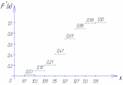 |
| Interval | 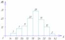 | 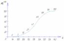 | 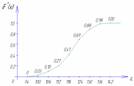 |
For graphical representation of variation series, the most commonly used are polygon, histogram, cumulative curve and empirical distribution function.
In table 2.3 (Grouping of the Russian population by average per capita income in April 1994) is presented interval variation series.
It is convenient to analyze distribution series using a graphical image, which allows one to judge the shape of the distribution. A visual representation of the nature of changes in the frequencies of the variation series is given by polygon and histogram.
The polygon is used when depicting discrete variation series.
Let us, for example, graphically depict the distribution of housing stock by type of apartment (Table 2.10).
Table 2.10 - Distribution of the housing stock of the urban area by type of apartment (conditional figures).

Rice. Housing distribution area
Not only the frequency values, but also the frequencies of the variation series can be plotted on the ordinate axes.
The histogram is used to depict an interval variation series. When constructing a histogram, the values of the intervals are plotted on the abscissa axis, and the frequencies are depicted by rectangles built on the corresponding intervals. The height of the columns in the case of equal intervals should be proportional to the frequencies. A histogram is a graph in which a series is depicted as bars adjacent to each other.
Let us graphically depict the interval distribution series given in table. 2.11.
Table 2.11 - Distribution of families by size of living space per person (conditional figures).
| N p/p | Groups of families by size of living space per person | Number of families with a given size of living space | Cumulative number of families |
| 1 | 3 – 5 | 10 | 10 |
| 2 | 5 – 7 | 20 | 30 |
| 3 | 7 – 9 | 40 | 70 |
| 4 | 9 – 11 | 30 | 100 |
| 5 | 11 – 13 | 15 | 115 |
| TOTAL | 115 | ---- | |

Rice. 2.2. Histogram of the distribution of families by the size of living space per person
Using the data of the accumulated series (Table 2.11), we construct cumulate distribution.

Rice. 2.3. Cumulative distribution of families by size of living space per person
The representation of a variation series in the form of a cumulate is especially effective for variation series whose frequencies are expressed as fractions or percentages of the sum of the series frequencies.
If we change the axes when graphically depicting a variation series in the form of cumulates, then we get ogiva. In Fig. 2.4 shows an ogive constructed on the basis of the data in Table. 2.11.
A histogram can be converted into a distribution polygon by finding the midpoints of the sides of the rectangles and then connecting these points with straight lines. The resulting distribution polygon is shown in Fig. 2.2 with a dotted line.
When constructing a histogram of the distribution of a variation series with unequal intervals, it is not the frequencies that are plotted along the ordinate, but the distribution density of the characteristic in the corresponding intervals.
The distribution density is the frequency calculated per unit interval width, i.e. how many units in each group are per unit of interval value. An example of calculating the distribution density is presented in table. 2.12.
Table 2.12 - Distribution of enterprises by number of employees (conditional figures)
| N p/p | Groups of enterprises by number of employees, people. | Number of enterprises | Interval size, people. | Distribution density |
| A | 1 | 2 | 3=1/2 | |
| 1 | Up to 20 | 15 | 20 | 0,75 |
| 2 | 20 – 80 | 27 | 60 | 0,25 |
| 3 | 80 – 150 | 35 | 70 | 0,5 |
| 4 | 150 – 300 | 60 | 150 | 0,4 |
| 5 | 300 – 500 | 10 | 200 | 0,05 |
| TOTAL | 147 | ---- | ---- |
Can also be used for graphical representation of variation series cumulative curve. Using a cumulate (sum curve), a series of accumulated frequencies is depicted. Cumulative frequencies are determined by sequentially summing frequencies across groups and show how many units in the population have attribute values no greater than the value under consideration.

Rice. 2.4. Ogive of distribution of families by the size of living space per person
When constructing the cumulate of an interval variation series, variants of the series are plotted along the abscissa axis, and accumulated frequencies are plotted along the ordinate axis.
When constructing an interval distribution series, three questions are resolved:
- 1. How many intervals should I take?
- 2. What is the length of the intervals?
- 3. What is the procedure for including population units within the boundaries of intervals?
- 1. Number of intervals can be determined by Sturgess formula:
2. Interval length, or interval step, usually determined by the formula
Where R- range of variation.
3. The order of inclusion of population units within the boundaries of the interval
may be different, but when constructing an interval series, the distribution must be strictly defined.
For example, this: [), in which population units are included in the lower boundaries, but are not included in the upper boundaries, but are transferred to the next interval. The exception to this rule is the last interval, the upper limit of which includes the last number of the ranked series.
The interval boundaries are:
- closed - with two extreme values of the attribute;
- open - with one extreme value of the attribute (before such and such a number or over such and such a number).
In order to assimilate the theoretical material, we introduce background information for solutions end-to-end task.
There are conditional data on the average number of sales managers, the quantity of similar goods sold by them, the individual market price for this product, as well as the sales volume of 30 companies in one of the regions of the Russian Federation in the first quarter of the reporting year (Table 2.1).
Table 2.1
Initial information for a cross-cutting task
|
Number managers, |
Price, thousand rubles |
Sales volume, million rubles. |
||
|
Number managers, |
Quantity of goods sold, pcs. |
Price, thousand rubles |
Sales volume, million rubles. |
|
Based on the initial information, as well as additional information, we will set up individual tasks. Then we will present the methodology for solving them and the solutions themselves.
Cross-cutting task. Task 2.1
Using the initial data from table. 2.1 required construct a discrete series of distribution of firms by quantity of goods sold (Table 2.2).
Solution:
Table 2.2
Discrete series of distribution of firms by quantity of goods sold in one of the regions of the Russian Federation in the first quarter of the reporting year
Cross-cutting task. Task 2.2
required construct a ranked series of 30 firms according to the average number of managers.
Solution:
15; 17; 18; 20; 20; 20; 22; 22; 24; 25; 25; 25; 27; 27; 27; 28; 29; 30; 32; 32; 33; 33; 33; 34; 35; 35; 38; 39; 39; 45.
Cross-cutting task. Task 2.3
Using the initial data from table. 2.1, required:
- 1. Construct an interval series of distribution of firms by number of managers.
- 2. Calculate the frequencies of the distribution series of firms.
- 3. Draw conclusions.
Solution:
Let's calculate using the Sturgess formula (2.5) number of intervals:
Thus, we take 6 intervals (groups).
Interval length, or interval step, calculate using the formula
Note. The order of inclusion of population units in the boundaries of the interval is as follows: I), in which population units are included in the lower boundaries, but are not included in the upper boundaries, but are transferred to the next interval. The exception to this rule is the last interval I ], the upper limit of which includes the last number of the ranked series.
We build an interval series (Table 2.3).
Interval series of distribution of firms and the average number of managers in one of the regions of the Russian Federation in the first quarter of the reporting year
Conclusion. The largest group of firms is the group with an average number of managers of 25-30 people, which includes 8 firms (27%); The smallest group with an average number of managers of 40-45 people includes only one company (3%).
Using the initial data from table. 2.1, as well as an interval series of distribution of firms by number of managers (Table 2.3), required build an analytical grouping of the relationship between the number of managers and the sales volume of firms and, based on it, draw a conclusion about the presence (or absence) of a relationship between these characteristics.
Solution:
Analytical grouping is based on factor characteristics. In our problem, the factor characteristic (x) is the number of managers, and the resultant characteristic (y) is the sales volume (Table 2.4).
Let's build now analytical grouping(Table 2.5).
Conclusion. Based on the data of the constructed analytical grouping, we can say that with an increase in the number of sales managers, the average sales volume of the company in the group also increases, which indicates the presence of a direct connection between these characteristics.
Table 2.4
Auxiliary table for constructing an analytical grouping
|
Number of managers, people, |
Company number |
Sales volume, million rubles, y |
|
|
" = 59 f = 9.97 |
|||
|
I-™ 4 - Yu.22 |
|||
|
74 '25 1PY1 U4 = 7 = 10,61 |
|||
|
at = ’ =10,31 30 |
|||
Table 2.5
Dependence of sales volumes on the number of company managers in one of the regions of the Russian Federation in the first quarter of the reporting year
CONTROL QUESTIONS- 1. What is the essence of statistical observation?
- 2. Name the stages of statistical observation.
- 3. What are the organizational forms of statistical observation?
- 4. Name the types of statistical observation.
- 5. What is a statistical summary?
- 6. Name the types of statistical reports.
- 7. What is statistical grouping?
- 8. Name the types of statistical groupings.
- 9. What is a distribution series?
- 10. Name the structural elements of the distribution row.
- 11. What is the procedure for constructing a distribution series?
Subject of mathematical statistics. General and sample population.
Math statistics– a branch of mathematics that studies methods of selecting, grouping, systematizing and analyzing statistical data to obtain scientifically based conclusions.
Statistical data– numerical values of the considered characteristic of the studied objects, obtained as a result of a random experiment.
Mathematical statistics is closely related to probability theory, but unlike probability theory, the mathematical model of the experiment is unknown. In mathematical statistics, using statistical data, it is necessary to establish an unknown probability distribution or objectively estimate the parameters of the distribution.
Methods of mathematical statistics make it possible to build optimal mathematical models of mass, repeating phenomena. The link between probability theory and mathematical statistics is the limit theorems of probability theory.
Currently, statistical methods are used in almost all sectors of the national economy.
Population– statistical data of all studied objects (sometimes – the objects themselves). Often the general population is considered as SV X.
Sample(sample population) – statistical data of objects selected randomly from the general population.
Sample size n(volume of the general population N) – the number of objects selected for study from the general population (the number of objects in the general population).
Examples.
A) Statistical data may be: student growth; the number of verbs (or other parts of speech) in a text passage of a certain length; GPA; level of intelligence; number of errors made by the dispatcher, etc.
b) General population maybe: the height of all people, the ranks of all factory workers, the frequency of use of a certain part of speech in all the works of the author being studied, the average grade point of the certificate of all graduates, etc.
V) Sampling could be: – the height of 20 students, the number of verbs in randomly selected 50 homogeneous passages of text with a length of 500 word usages, the average grade point of the certificate of 100 graduates randomly selected from city schools, etc.
The sample is called representative if it correctly reflects the property of the general population. Representativeness of the sample is achieved by random selection, when all objects in the population have the same probability of being selected.
In order for the sample to be representative, various methods of selecting objects of study are used.
Types of selection: simple, mechanical, serial, typical.
Simple. Elements are randomly selected from the entire population.
Mechanical selection. Every 10 (25, 30, etc.) object from the general population is selected.
Serial. A study is carried out in each series (for example, 10 passages of 500 word uses are selected from the text - 10 series).
Typical. The general population is divided into typical groups according to a certain characteristic. The number of series extracted from each such group is determined by the proportion of this group in the general population.
Statistical distribution of the sample and its graphical representation.
Let us study the SV X (general population) with respect to some characteristic. A number of independent tests are being carried out. As a result of the experiments, SV X takes on certain values. The set of obtained values represents a sample, and the values themselves are statistical data.
Initially, the sample is ranked - the statistical data of the sample is arranged in non-decreasing order. We get a variation series.
Variation series- ranked sample.
Discrete statistical series
If the general population is a discrete SV, a discrete statistical series (statistical distribution) is constructed.
Let the value appear in the sample once,
Raza,..., - times.
I-th option samples; - frequency i-th option Frequency shows how many times a given option appeared in the sample.
- relative frequency i-th options
(shows what part of the sample is ).
A statistical distribution is the correspondence between sampling options and their frequencies or relative frequencies.
For DSV, the statistical distribution can be presented in the form of a table - a statistical series of frequencies or a statistical series of relative frequencies.
Statistical series of frequencies Statistical series
relative frequencies
| ........ | ||||
| ........ |
| ........ | ||||
| ........ |
To visualize the statistical distribution of the sample, “graphs” of the statistical distribution are constructed: a polygon and a histogram.
Frequency polygon(relative frequencies) – a graphical representation of a discrete statistical series - a broken line sequentially connecting points [for a polygon of relative frequencies].
Example. The researcher is interested in the mathematics knowledge of applicants. 10 applicants are selected and their school grades in this subject are recorded. The following sample was obtained: 5;4;4;3;2;5;4;3;4;5.
a) Present the sample in the form of a variation series;
b) construct a statistical series of frequencies and relative frequencies;
c) draw a polygon of relative frequencies for the resulting series.
a) Let's rank the sample, i.e. Let's arrange the sample members in non-decreasing order. We get the variation series: 2; 3; 3; 4; 4; 4; 4; 5; 5;5.
b) Construct a statistical series of frequencies (correspondence between sampling options and their frequencies) and a statistical series of relative frequencies (correspondence between sampling options and their relative frequencies)
| 0,1 | 0,2 | 0,4 | 0,3 |
Statistical frequency series statistical series rel. frequencies
1+2+4+3=10=n 0.1+0.2+0.4+0.3=1.
Relative frequency polygon.


