Expansion of a periodic function into a trigonometric Fourier series. Fourier series expansion in cosines

Which are already pretty boring. And I feel that the moment has come when it is time to extract new canned goods from the strategic reserves of theory. Is it possible to expand the function into a series in some other way? For example, express a straight line segment in terms of sines and cosines? It seems incredible, but such seemingly distant functions can be
"reunification". In addition to the familiar degrees in theory and practice, there are other approaches to expanding a function into a series.

In this lesson we will learn about trigonometry. near Fourier, we will touch on the issue of its convergence and sum and, of course, we will analyze numerous examples of the expansion of functions in a Fourier series. I sincerely wanted to call the article “Fourier Series for Dummies,” but this would be disingenuous, since solving the problems would require knowledge of other branches of mathematical analysis and some practical experience. Therefore, the preamble will resemble astronaut training =)

Firstly, you should approach the study of page materials in excellent form. Sleepy, rested and sober. Without strong emotions about a broken hamster's paw and obsessive thoughts about the hardships of life aquarium fish. The Fourier series is not difficult to understand, however practical tasks they simply require increased concentration of attention - ideally, you should completely detach yourself from external stimuli. The situation is aggravated by the fact that there is no easy way to check the solution and answer. Thus, if your health is below average, then it is better to do something simpler. Is it true.

Secondly, before flying into space you need to study the instrument panel spaceship. Let's start with the values ​​of the functions that should be clicked on the machine:

For any natural value:

1) . Indeed, the sinusoid “stitches” the x-axis through each “pi”:
. In the case of negative values ​​of the argument, the result, of course, will be the same: .

2) . But not everyone knew this. The cosine "pi" is the equivalent of a "blinker":

A negative argument does not change the matter: .

Perhaps that's enough.

And thirdly, dear cosmonaut corps, you must be able to... integrate.
In particular, confidently subsume a function under the differential sign, integrate by parts and be in harmony with the Newton-Leibniz formula. Let's begin the important pre-flight exercises. I categorically do not recommend skipping it, so as not to squish in weightlessness later:

Example 1

Calculate definite integrals

where takes natural values.

Solution: integration is carried out over the variable “x” and at this stage the discrete variable “en” is considered a constant. In all integrals we subsume the function under the differential sign:

A short version of the solution that would be good to target looks like this:

Let's get used to it:

The four remaining points are on your own. Try to approach the task conscientiously and write the integrals in a short way. Sample solutions at the end of the lesson.

After performing the exercises QUALITY, we put on spacesuits
and getting ready to start!

Expansion of a function into a Fourier series on the interval

Let's consider some function that is defined at least on an interval (and, possibly, on a larger interval). If this function is integrable on the interval, then it can be expanded into a trigonometric Fourier series:
, where are the so-called Fourier coefficients.

In this case, the number is called the decomposition period, and the number is called the decomposition half-period.

It is obvious that in the general case the Fourier series consists of sines and cosines:

Indeed, let’s write it down in detail:

The zero term of the series is usually written in the form .

Fourier coefficients are calculated using the following formulas:

I understand perfectly well that those starting to study the topic are still unclear about the new terms: decomposition period, half-cycle, Fourier coefficients etc. Don’t panic, this is not comparable to the excitement before going into outer space. Let’s understand everything in the following example, before executing which it is logical to ask pressing practical questions:

What do you need to do in the following tasks?

Expand the function into a Fourier series. Additionally, it is often necessary to depict a graph of a function, a graph of the sum of a series, a partial sum, and in the case of sophisticated professorial fantasies, do something else.

How to expand a function into a Fourier series?

Essentially, you need to find Fourier coefficients, that is, compose and calculate three definite integrals.

Please rewrite the general form of the Fourier series and the three working formulas in your notebook. I am very glad that some site visitors are realizing their childhood dream of becoming an astronaut right before my eyes =)

Example 2

Expand the function into a Fourier series on the interval. Construct a graph, a graph of the sum of the series and the partial sum.

Solution: The first part of the task is to expand the function into a Fourier series.

The beginning is standard, be sure to write down that:

In this problem, the expansion period is half-period.

Let us expand the function into a Fourier series on the interval:

Using the appropriate formulas, we find Fourier coefficients. Now you need to compose and calculate three definite integrals. For convenience, I will number the points:

1) The first integral is the simplest, however, it also requires eyeballs:

2) Use the second formula:

This integral is well known and is taken in parts:

When finding, the method of subsuming the function under the differential sign was used.

In the task under consideration, it is more convenient to immediately use the formula for integration by parts in a definite integral :

A couple of technical notes. Firstly, after applying the formula, the entire expression must be enclosed in large brackets, since there is a constant in front of the original integral. Let's not lose her! The parentheses can be expanded at any further step; I did this as a last resort. In the first "piece" We show extreme care in the substitution; as you can see, the constant is not used, and the limits of integration are substituted into the product. This action is highlighted in square brackets. Well, you are familiar with the integral of the second “piece” of the formula from the training task;-)

And most importantly - extreme concentration!

3) We are looking for the third Fourier coefficient:

A relative of the previous integral is obtained, which can also be integrated by parts:

This instance is a little more complicated, I’ll comment on the further steps step by step:

(1) We enclose the entire expression in large brackets. I didn’t want to seem boring, they lose the constant too often.

(2) V in this case I immediately opened those big brackets. Special attention We devote ourselves to the first “piece”: the constant smokes on the sidelines and does not participate in the substitution of the limits of integration ( and ) into the product . Due to the clutter of the record, it is again advisable to highlight this action with square brackets. With the second "piece" everything is simpler: here the fraction appeared after opening large parentheses, and the constant - as a result of integrating the familiar integral;-)

(3) In square brackets we carry out transformations, and in the right integral - substitution of integration limits.

(4) We remove the “flashing light” from the square brackets: , and then open the inner brackets: .

(5) We cancel 1 and –1 in brackets and make final simplifications.

Finally, all three Fourier coefficients are found:

Let's substitute them into the formula :

At the same time, do not forget to divide in half. At the last step, the constant (“minus two”), which does not depend on “en,” is taken outside the sum.

Thus, we have obtained the expansion of the function into a Fourier series on the interval:

Let us study the issue of convergence of the Fourier series. I will explain the theory, in particular Dirichlet's theorem, literally "on the fingers", so if you need strict formulations, please refer to the textbook on mathematical analysis (for example, the 2nd volume of Bohan; or the 3rd volume of Fichtenholtz, but it is more difficult).

The second part of the problem requires drawing a graph, a graph of the sum of a series, and a graph of a partial sum.

The graph of the function is an ordinary straight line on the plane, which is drawn with a black dotted line:

Let's figure out the sum of the series. As you know, function series converge to functions. In our case, the constructed Fourier series for any value of "x" will converge to the function, which is shown in red. This function suffers discontinuities of the 1st kind at points , but is also defined at them (red dots in the drawing)

Thus: . It is easy to see that it is noticeably different from the original function, which is why in the entry A tilde is used rather than an equals sign.

Let's study an algorithm that is convenient for constructing the sum of a series.

On the central interval, the Fourier series converges to the function itself (the central red segment coincides with the black dotted line of the linear function).

Now let's talk a little about the nature of the trigonometric expansion under consideration. Fourier series includes only periodic functions (constant, sines and cosines), so the sum of the series is also a periodic function.

What does this mean in our specific example? And this means that the sum of the series – is certainly periodic and the red segment of the interval must be repeated endlessly on the left and right.

I think the meaning of the phrase “period of decomposition” has now finally become clear. To put it simply, every time the situation repeats itself again and again.

In practice, it is usually sufficient to depict three periods of decomposition, as is done in the drawing. Well, and also “stumps” of neighboring periods - so that it is clear that the graph continues.

Of particular interest are discontinuity points of the 1st kind. At such points, the Fourier series converges to isolated values, which are located exactly in the middle of the “jump” of the discontinuity (red dots in the drawing). How to find out the ordinate of these points? First, let’s find the ordinate of the “upper floor”: to do this, we calculate the value of the function at the rightmost point of the central period of the expansion: . To calculate the ordinate of the “lower floor” the easiest way is to take the extreme left value of the same period: . The ordinate of the average value is the arithmetic mean of the sum of “top and bottom”: . A pleasant fact is that when constructing a drawing, you will immediately see whether the middle is calculated correctly or incorrectly.

Let’s construct a partial sum of the series and at the same time repeat the meaning of the term “convergence.” The motif is also known from the lesson on the sum of a number series. Let us describe our wealth in detail:

To compose a partial sum, you need to write zero + two more terms of the series. That is,

The drawing shows the graph of the function green, and, as you can see, it “wraps” the full amount quite tightly. If we consider a partial sum of five terms of the series, then the graph of this function will approximate the red lines even more accurately; if there are one hundred terms, then the “green serpent” will actually completely merge with the red segments, etc. Thus, the Fourier series converges to its sum.

It is interesting to note that any partial sum is a continuous function, but the total sum of the series is still discontinuous.

In practice, it is not so rare to construct a partial sum graph. How to do it? In our case, it is necessary to consider the function on the segment, calculate its values ​​at the ends of the segment and at intermediate points (the more points you consider, the more accurate the graph will be). Then you should mark these points on the drawing and carefully draw a graph on the period, and then “replicate” it into adjacent intervals. How else? After all, approximation is also a periodic function... ...in some ways its graph reminds me of a smooth heart rhythm on the display of a medical device.

Carrying out the construction, of course, is not very convenient, since you have to be extremely careful, maintaining an accuracy of no less than half a millimeter. However, I will please readers who are not comfortable with drawing - in a “real” problem it is not always necessary to carry out a drawing; in about 50% of cases it is necessary to expand the function into a Fourier series and that’s it.

After completing the drawing, we complete the task:

Answer :

In many problems, the function suffers a discontinuity of the 1st kind right at the expansion period:

Example 3

Expand the function given on the interval into a Fourier series. Draw a graph of the function and the total sum of the series.

The proposed function is specified in a piecewise manner (and, note, only on the segment) and suffers a discontinuity of the 1st kind at the point . Is it possible to calculate Fourier coefficients? No problem. Both the left and right sides of the function are integrable on their intervals, therefore the integrals in each of the three formulas should be represented as the sum of two integrals. Let's see, for example, how this is done for a zero coefficient:

The second integral turned out to be equal to zero, which reduced the work, but this is not always the case.

The other two Fourier coefficients are described similarly.

How to show the sum of a series? On the left interval we draw a straight line segment, and on the interval - a straight line segment (we highlight the section of the axis in bold and bold). That is, on the expansion interval, the sum of the series coincides with the function everywhere except for three “bad” points. At the discontinuity point of the function, the Fourier series will converge to an isolated value, which is located exactly in the middle of the “jump” of the discontinuity. It is not difficult to see it orally: left-sided limit: , right-sided limit: and, obviously, the ordinate of the midpoint is 0.5.

Due to the periodicity of the sum, the picture must be “multiplied” into adjacent periods, in particular, the same thing must be depicted on the intervals and . At the same time, at points the Fourier series will converge to the median values.

In fact, there is nothing new here.

Try to cope with this task yourself. An approximate sample of the final design and a drawing at the end of the lesson.

Expansion of a function into a Fourier series over an arbitrary period

For an arbitrary expansion period, where “el” is any positive number, the formulas for the Fourier series and Fourier coefficients are distinguished by a slightly more complicated argument for sine and cosine:

If , then we get the interval formulas with which we started.

The algorithm and principles for solving the problem are completely preserved, but the technical complexity of the calculations increases:

Example 4

Expand the function into a Fourier series and plot the sum.

Solution: actually an analogue of Example No. 3 with a discontinuity of the 1st kind at the point. In this problem, the expansion period is half-period. The function is defined only on the half-interval, but this does not change the matter - it is important that both pieces of the function are integrable.

Let's expand the function into a Fourier series:

Since the function is discontinuous at the origin, each Fourier coefficient should obviously be written as the sum of two integrals:

1) I will write out the first integral in as much detail as possible:

2) We carefully look at the surface of the Moon:

We take the second integral by parts:

What should we pay close attention to after we open the continuation of the solution with an asterisk?

Firstly, we do not lose the first integral , where we immediately apply the differential sign. Secondly, do not forget the ill-fated constant before large brackets and do not get confused in the signs when using the formula . Large brackets are still more convenient to open immediately in the next step.

The rest is a matter of technique; difficulties can only be caused by insufficient experience in solving integrals.

Yes, it was not for nothing that the eminent colleagues of the French mathematician Fourier were indignant - how did he dare to arrange functions into trigonometric series?! =) By the way, everyone is probably interested in the practical meaning of the task in question. Fourier himself worked on mathematical model thermal conductivity, and subsequently the series named after him began to be used to study many periodic processes, which are visible and invisible in the surrounding world. Now, by the way, I caught myself thinking that it was not by chance that I compared the graph of the second example with the periodic rhythm of the heart. Those interested can familiarize themselves with the practical application Fourier transform in third party sources. ...Although it’s better not to - it will be remembered as First Love =)

3) Taking into account the repeatedly mentioned weak links, let’s look at the third coefficient:

Let's integrate by parts:

Let us substitute the found Fourier coefficients into the formula , not forgetting to divide the zero coefficient in half:

Let's plot the sum of the series. Let us briefly repeat the procedure: we construct a straight line on an interval, and a straight line on an interval. If the “x” value is zero, we put a point in the middle of the “jump” of the gap and “replicate” the graph for adjacent periods:


At the “junctions” of periods, the sum will also be equal to the midpoints of the “jump” of the gap.

Ready. Let me remind you that the function itself is by condition defined only on a half-interval and, obviously, coincides with the sum of the series on the intervals

Answer :

Sometimes a piecewise given function is continuous over the expansion period. The simplest example: . Solution (see Bohan volume 2) the same as in the two previous examples: despite the continuity of the function at the point, each Fourier coefficient is expressed as the sum of two integrals.

In the expansion interval, there may be more discontinuity points of the 1st kind and/or “joint” points of the graph (two, three, and generally any final quantity). If a function is integrable on each part, then it is also expandable in a Fourier series. But from practical experience I don’t remember such a cruel thing. However, there are more difficult tasks than those just considered, and at the end of the article there are links to Fourier series of increased complexity for everyone.

In the meantime, let’s relax, lean back in our chairs and contemplate the endless expanses of stars:

Example 5

Expand the function into a Fourier series on the interval and plot the sum of the series.

In this problem, the function is continuous on the half-interval of the expansion, which simplifies the solution. Everything is very similar to Example No. 2. There's no escape from the spaceship - you'll have to decide =) An approximate design sample at the end of the lesson, a schedule is attached.

Fourier series expansion of even and odd functions

With even and odd functions, the process of solving the problem is noticeably simplified. And that's why. Let's return to the expansion of a function in a Fourier series with a period of “two pi” and arbitrary period “two el” .

Let's assume that our function is even. The general term of the series, as you can see, contains even cosines and odd sines. And if we are expanding an EVEN function, then why do we need odd sines?! Let's reset the unnecessary coefficient: .

Thus, an even function can be expanded into a Fourier series only in cosines:

Since the integrals of even functions over an integration segment that is symmetrical with respect to zero can be doubled, the remaining Fourier coefficients are also simplified.

For the gap:

For an arbitrary interval:

Textbook examples that can be found in almost any textbook on mathematical analysis include expansions of even functions . In addition, they have been encountered several times in my personal practice:

Example 6

The function is given. Required:

1) expand the function into a Fourier series with period , where is an arbitrary positive number;

2) write down the expansion on the interval, construct a function and graph the total sum of the series.

Solution: in the first paragraph it is proposed to solve the problem in general view, and it's very convenient! If the need arises, just substitute your value.

1) In this problem, the expansion period is half-period. During further actions, in particular during integration, "el" is considered a constant

The function is even, which means it can be expanded into a Fourier series only in cosines: .

We look for Fourier coefficients using the formulas . Pay attention to their unconditional advantages. Firstly, the integration is carried out over the positive segment of the expansion, which means we safely get rid of the module , considering only the “X” of the two pieces. And, secondly, integration is noticeably simplified.

Two:

Let's integrate by parts:

Thus:
, while the constant , which does not depend on “en”, is taken outside the sum.

Answer :

2) Let us write the expansion on the interval, for this purpose in general formula substitute desired value half cycle:

Fourier series are a representation of an arbitrary function with a specific period in the form of a series. In general, this solution is called the decomposition of an element along an orthogonal basis. Expansion of functions into Fourier series is a fairly powerful tool for solving various problems due to the properties of this transformation during integration, differentiation, as well as shifting expressions by argument and convolution.

A person who is not familiar with higher mathematics, as well as with the works of the French scientist Fourier, most likely will not understand what these “series” are and what they are needed for. Meanwhile, this transformation has become quite integrated into our lives. It is used not only by mathematicians, but also by physicists, chemists, doctors, astronomers, seismologists, oceanographers and many others. Let us also take a closer look at the works of the great French scientist who made a discovery that was ahead of its time.

Man and the Fourier transform

Fourier series are one of the methods (along with analysis and others). This process occurs every time a person hears a sound. Our ear automatically carries out the transformation elementary particles in an elastic medium are laid out in rows (along the spectrum) of successive loudness level values ​​for tones of different heights. Next, the brain turns this data into sounds that are familiar to us. All this happens without our desire or consciousness, on its own, but in order to understand these processes, it will take several years to study higher mathematics.

More about Fourier transform

The Fourier transform can be carried out using analytical, numerical and other methods. Fourier series refer to the numerical method of decomposing any oscillatory processes - from ocean tides and light waves to cycles of solar (and other astronomical objects) activity. Using these mathematical techniques, you can analyze functions, representing any oscillatory processes as a series of sinusoidal components that move from minimum to maximum and back. The Fourier transform is a function that describes the phase and amplitude of sinusoids corresponding to a specific frequency. This process can be used to solve very complex equations that describe dynamic processes arising under the influence of heat, light or electrical energy. Also, Fourier series make it possible to isolate constant components in complex oscillatory signals, making it possible to correctly interpret the experimental observations obtained in medicine, chemistry and astronomy.

Historical reference

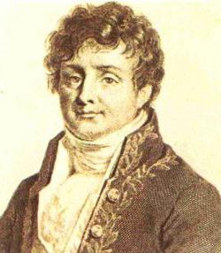
The founding father of this theory is the French mathematician Jean Baptiste Joseph Fourier. This transformation was subsequently named after him. Initially, the scientist used his method to study and explain the mechanisms of thermal conductivity - the spread of heat in solids. Fourier suggested that the initial irregular distribution can be decomposed into simple sinusoids, each of which will have its own temperature minimum and maximum, as well as its own phase. In this case, each such component will be measured from minimum to maximum and back. The mathematical function that describes the upper and lower peaks of the curve, as well as the phase of each of the harmonics, is called the Fourier transform of the temperature distribution expression. The author of the theory brought together general function distribution, which is difficult to describe mathematically, to a very convenient series of cosine and sine, which together give the original distribution.

The principle of transformation and the views of contemporaries

The scientist's contemporaries - leading mathematicians of the early nineteenth century - did not accept this theory. The main objection was Fourier's assertion that a discontinuous function, describing a straight line or a discontinuous curve, can be represented as a sum of sinusoidal expressions that are continuous. As an example, consider the Heaviside step: its value is zero to the left of the discontinuity and one to the right. This function describes the dependence of the electric current on a temporary variable when the circuit is closed. Contemporaries of the theory at that time had never encountered a similar situation where a discontinuous expression would be described by a combination of continuous, ordinary functions such as exponential, sine, linear or quadratic.

What confused French mathematicians about Fourier's theory?

After all, if the mathematician was right in his statements, then by summing the infinite trigonometric Fourier series, one can obtain an accurate representation of the step expression even if it has many similar steps. At the beginning of the nineteenth century, such a statement seemed absurd. But despite all the doubts, many mathematicians expanded the scope of study of this phenomenon, taking it beyond the study of thermal conductivity. However, most scientists continued to be tormented by the question: “Can the sum of a sinusoidal series converge to exact value discontinuous function?

Convergence of Fourier series: an example

The question of convergence arises whenever it is necessary to sum infinite series of numbers. To understand this phenomenon, consider a classic example. Will you ever be able to reach the wall if each subsequent step is half the size of the previous one? Let's say you're two meters from your target, the first step takes you to the halfway mark, the next one takes you to the three-quarters mark, and after the fifth you'll have covered almost 97 percent of the way. However, no matter how many steps you take, you will not achieve your intended goal in a strict mathematical sense. Using numerical calculations, it can be proven that it is eventually possible to get as close as a given distance. This proof is equivalent to demonstrating that the sum of one-half, one-fourth, etc. will tend to one.

The Question of Convergence: The Second Coming, or Lord Kelvin's Instrument

This issue was raised again at the end of the nineteenth century, when they tried to use Fourier series to predict the intensity of tides. At this time, Lord Kelvin invented a device that was an analog computing device, which allowed military and merchant marine sailors to track this natural phenomenon. This mechanism determined sets of phases and amplitudes from a table of tide heights and corresponding time points, carefully measured in a given harbor throughout the year. Each parameter was a sinusoidal component of the tide height expression and was one of the regular components. The measurements were fed into Lord Kelvin's calculating instrument, which synthesized a curve that predicted the height of the water as a function of time for the following year. Very soon similar curves were drawn up for all the harbors of the world.

What if the process is disrupted by a discontinuous function?

At that time it seemed obvious that a tidal wave predictor with a large number of counting elements could calculate a large number of phases and amplitudes and thus provide more accurate predictions. However, it turned out that this pattern is not observed in cases where the tidal expression that should be synthesized contained a sharp jump, that is, it was discontinuous. If data from a table of time moments is entered into the device, it calculates several Fourier coefficients. The original function is restored thanks to the sinusoidal components (in accordance with the found coefficients). The discrepancy between the original and reconstructed expression can be measured at any point. When carrying out repeated calculations and comparisons, it is clear that the value of the largest error does not decrease. However, they are localized in the region corresponding to the discontinuity point, and at any other point they tend to zero. In 1899, this result was theoretically confirmed by Joshua Willard Gibbs of Yale University.

Convergence of Fourier series and the development of mathematics in general

Fourier analysis is not applicable to expressions containing an infinite number of spikes over a certain interval. In general, Fourier series, if the original function is represented by the result of the real physical dimension, always converge. Questions about the convergence of this process for specific classes of functions led to the emergence of new branches in mathematics, for example, the theory of generalized functions. She is associated with such names as L. Schwartz, J. Mikusinski and J. Temple. Within the framework of this theory, a clear and precise theoretical basis under such expressions as the Dirac delta function (it describes a region of a single area concentrated in an infinitesimal neighborhood of a point) and the Heaviside “step”. Thanks to this work, Fourier series became applicable to solving equations and problems involving intuitive concepts: point charge, point mass, magnetic dipoles, and concentrated load on a beam.

Fourier method

Fourier series, in accordance with the principles of interference, begin with the decomposition of complex forms into simpler ones. For example, a change in heat flow is explained by its passage through various obstacles made of heat-insulating material of irregular shape or a change in the surface of the earth - an earthquake, a change in orbit celestial body- influence of planets. As a rule, such equations that describe simple classical systems can be easily solved for each individual wave. Fourier showed that simple solutions can also be summed to obtain solutions to more complex problems. In mathematical terms, Fourier series are a technique for representing an expression as a sum of harmonics - cosine and sine. That's why this analysis also known as harmonic analysis.

Fourier series - an ideal technique before the “computer age”

Before creation computer equipment The Fourier technique was the best weapon in the arsenal of scientists when working with the wave nature of our world. Fourier series complex form allows you to decide not only simple tasks, which are amenable to the direct application of Newton's laws of mechanics, but also fundamental equations. Most of the discoveries of Newtonian science in the nineteenth century were made possible only by Fourier's technique.

Fourier series today

With the development of computers, Fourier transforms have risen to a qualitatively new level. This technique is firmly established in almost all areas of science and technology. An example is digital audio and video. Its implementation became possible only thanks to a theory developed by a French mathematician at the beginning of the nineteenth century. Thus, the Fourier series in a complex form made it possible to make a breakthrough in the study of outer space. In addition, it influenced the study of the physics of semiconductor materials and plasma, microwave acoustics, oceanography, radar, and seismology.

Trigonometric Fourier series

In mathematics, a Fourier series is a way of representing arbitrary complex functions the sum of simpler ones. IN general cases the number of such expressions can be infinite. Moreover, the more their number is taken into account in the calculation, the more accurate the final result is. Most often used as protozoa trigonometric functions cosine or sine. In this case, Fourier series are called trigonometric, and the solution of such expressions is called harmonic expansion. This method plays important role in mathematics. First of all, the trigonometric series provides a means for depicting and also studying functions; it is the main apparatus of the theory. In addition, it allows you to solve a number of problems in mathematical physics. Finally, this theory contributed to the development and brought to life a number of very important sections mathematical science(theory of integrals, theory of periodic functions). In addition, it served as the starting point for the development of the following functions of a real variable, and also laid the foundation for harmonic analysis.

Fourier series of periodic functions with period 2π.

The Fourier series allows us to study periodic functions by decomposing them into components. Alternating currents and voltages, displacements, speed and acceleration of crank mechanisms and acoustic waves are typical practical examples application of periodic functions in engineering calculations.

The Fourier series expansion is based on the assumption that all functions of practical significance in the interval -π ≤x≤ π can be expressed in the form of convergent trigonometric series (a series is considered convergent if the sequence of partial sums composed of its terms converges):

Standard (=ordinary) notation through the sum of sinx and cosx

f(x)=a o + a 1 cosx+a 2 cos2x+a 3 cos3x+...+b 1 sinx+b 2 sin2x+b 3 sin3x+...,

where a o, a 1,a 2,...,b 1,b 2,.. are real constants, i.e.

Where, for the range from -π to π, the coefficients of the Fourier series are calculated using the formulas:

The coefficients a o , a n and b n are called Fourier coefficients, and if they can be found, then series (1) is called the Fourier series corresponding to the function f (x). For series (1), the term (a 1 cosx+b 1 sinx) is called the first or fundamental harmonic,

Another way to write a series is to use the relation acosx+bsinx=csin(x+α)

f(x)=a o +c 1 sin(x+α 1)+c 2 sin(2x+α 2)+...+c n sin(nx+α n)

Where a o is a constant, c 1 =(a 1 2 +b 1 2) 1/2, c n =(a n 2 +b n 2) 1/2 are the amplitudes of the various components, and is equal to a n =arctg a n /b n.

For series (1), the term (a 1 cosx+b 1 sinx) or c 1 sin(x+α 1) is called the first or fundamental harmonic, (a 2 cos2x+b 2 sin2x) or c 2 sin(2x+α 2) called the second harmonic and so on.

To accurately represent a complex signal typically requires an infinite number of terms. However, in many practical problems it is sufficient to consider only the first few terms.

Fourier series of non-periodic functions with period 2π.

Expansion of non-periodic functions.

If the function f(x) is non-periodic, it means that it cannot be expanded into a Fourier series for all values ​​of x. However, it is possible to define a Fourier series representing a function over any range of width 2π.

Given a non-periodic function, a new function can be constructed by selecting values ​​of f(x) within a certain range and repeating them outside that range at 2π intervals. Since the new function is periodic with period 2π, it can be expanded into a Fourier series for all values ​​of x. For example, the function f(x)=x is not periodic. However, if it is necessary to expand it into a Fourier series in the interval from o to 2π, then outside this interval a periodic function with a period of 2π is constructed (as shown in the figure below).

For non-periodic functions such as f(x)=x, the sum of the Fourier series is equal to the value of f(x) at all points in a given range, but it is not equal to f(x) for points outside the range. To find the Fourier series of a non-periodic function in the 2π range, the same formula of Fourier coefficients is used.

Even and odd functions.

They say a function y=f(x) is even if f(-x)=f(x) for all values ​​of x. Graphs of even functions are always symmetrical about the y-axis (that is, they are mirror images). Two examples of even functions: y=x2 and y=cosx.

A function y=f(x) is said to be odd if f(-x)=-f(x) for all values ​​of x. Graphs of odd functions are always symmetrical about the origin.

Many functions are neither even nor odd.

Fourier series expansion in cosines.

The Fourier series of an even periodic function f(x) with period 2π contains only cosine terms (i.e., no sine terms) and may include a constant term. Hence,

where are the coefficients of the Fourier series,

The Fourier series of an odd periodic function f(x) with period 2π contains only terms with sines (that is, it does not contain terms with cosines).

Hence,

where are the coefficients of the Fourier series,

Fourier series at half cycle.

If a function is defined for a range, say from 0 to π, and not just from 0 to 2π, it can be expanded in a series only in sines or only in cosines. The resulting Fourier series is called the half-cycle Fourier series.

If you want to obtain a half-cycle Fourier expansion of the cosines of the function f(x) in the range from 0 to π, then you need to construct an even periodic function. In Fig. Below is the function f(x)=x, built on the interval from x=0 to x=π. Because the even function symmetrical about the f(x) axis, draw line AB, as shown in Fig. below. If we assume that outside the considered interval the obtained triangular shape is periodic with a period of 2π, then the final graph looks like, show. in Fig. below. Since we need to obtain the Fourier expansion in cosines, as before, we calculate the Fourier coefficients a o and a n

If you want to obtain a half-cycle Fourier expansion in terms of the sines of the function f(x) in the range from 0 to π, then you need to construct an odd periodic function. In Fig. Below is the function f(x)=x, built on the interval from x=0 to x=π. Since the odd function is symmetrical about the origin, we construct the line CD, as shown in Fig. If we assume that outside the considered interval the resulting sawtooth signal is periodic with a period of 2π, then the final graph has the form shown in Fig. Since we need to obtain the Fourier expansion of the half-cycle in terms of sines, as before, we calculate the Fourier coefficient. b

Fourier series for an arbitrary interval.

Expansion of a periodic function with period L.

The periodic function f(x) repeats as x increases by L, i.e. f(x+L)=f(x). The transition from the previously considered functions with a period of 2π to functions with a period of L is quite simple, since it can be done using a change of variable.

To find the Fourier series of the function f(x) in the range -L/2≤x≤L/2, we introduce a new variable u so that the function f(x) has a period of 2π relative to u. If u=2πx/L, then x=-L/2 for u=-π and x=L/2 for u=π. Also let f(x)=f(Lu/2π)=F(u). The Fourier series F(u) has the form

(The limits of integration can be replaced by any interval of length L, for example, from 0 to L)

Fourier series on a half-cycle for functions specified in the interval L≠2π.

For the substitution u=πх/L, the interval from x=0 to x=L corresponds to the interval from u=0 to u=π. Consequently, the function can be expanded into a series only in cosines or only in sines, i.e. into a Fourier series at half cycle.

The cosine expansion in the range from 0 to L has the form

Functions, decomposing them into components. Alternating currents and voltages, displacements, speed and acceleration of crank mechanisms and acoustic waves are typical practical examples of the use of periodic functions in engineering calculations.

The Fourier series expansion is based on the assumption that all functions of practical significance in the interval -π ≤x≤ π can be expressed in the form of convergent trigonometric series (a series is considered convergent if the sequence of partial sums composed of its terms converges):

Standard (=ordinary) notation through the sum of sinx and cosx

f(x)=a o + a 1 cosx+a 2 cos2x+a 3 cos3x+...+b 1 sinx+b 2 sin2x+b 3 sin3x+...,

where a o, a 1,a 2,...,b 1,b 2,.. are real constants, i.e.

Where, for the range from -π to π, the coefficients of the Fourier series are calculated using the formulas:

The coefficients a o , a n and b n are called Fourier coefficients, and if they can be found, then series (1) is called the Fourier series corresponding to the function f (x). For series (1), the term (a 1 cosx+b 1 sinx) is called the first or fundamental harmonic,

Another way to write a series is to use the relation acosx+bsinx=csin(x+α)

f(x)=a o +c 1 sin(x+α 1)+c 2 sin(2x+α 2)+...+c n sin(nx+α n)

Where a o is a constant, c 1 =(a 1 2 +b 1 2) 1/2, c n =(a n 2 +b n 2) 1/2 are the amplitudes of the various components, and is equal to a n =arctg a n /b n.

For series (1), the term (a 1 cosx+b 1 sinx) or c 1 sin(x+α 1) is called the first or fundamental harmonic, (a 2 cos2x+b 2 sin2x) or c 2 sin(2x+α 2) called the second harmonic and so on.

To accurately represent a complex signal typically requires an infinite number of terms. However, in many practical problems it is sufficient to consider only the first few terms.

Fourier series of non-periodic functions with period 2π. Expansion of non-periodic functions into Fourier series.

If the function f(x) is non-periodic, it means that it cannot be expanded into a Fourier series for all values ​​of x. However, it is possible to define a Fourier series representing a function over any range of width 2π.

Given a non-periodic function, a new function can be constructed by selecting values ​​of f(x) within a certain range and repeating them outside that range at 2π intervals. Since the new function is periodic with period 2π, it can be expanded into a Fourier series for all values ​​of x. For example, the function f(x)=x is not periodic. However, if it is necessary to expand it into a Fourier series in the interval from o to 2π, then outside this interval a periodic function with a period of 2π is constructed (as shown in the figure below).

For non-periodic functions such as f(x)=x, the sum of the Fourier series is equal to the value of f(x) at all points in a given range, but it is not equal to f(x) for points outside the range. To find the Fourier series of a non-periodic function in the 2π range, the same formula of Fourier coefficients is used.

Even and odd functions.

They say a function y=f(x) is even if f(-x)=f(x) for all values ​​of x. Graphs of even functions are always symmetrical about the y-axis (that is, they are mirror images). Two examples of even functions: y=x2 and y=cosx.

A function y=f(x) is said to be odd if f(-x)=-f(x) for all values ​​of x. Graphs of odd functions are always symmetrical about the origin.

Many functions are neither even nor odd.

Fourier series expansion in cosines.

The Fourier series of an even periodic function f(x) with period 2π contains only cosine terms (i.e., no sine terms) and may include a constant term. Hence,

where are the coefficients of the Fourier series,

The Fourier series of an odd periodic function f(x) with period 2π contains only terms with sines (that is, it does not contain terms with cosines).

Hence,

where are the coefficients of the Fourier series,

Fourier series at half cycle.

If a function is defined for a range, say from 0 to π, and not just from 0 to 2π, it can be expanded in a series only in sines or only in cosines. The resulting Fourier series is called the half-cycle Fourier series.

If you want to obtain a half-cycle Fourier expansion of the cosines of the function f(x) in the range from 0 to π, then you need to construct an even periodic function. In Fig. Below is the function f(x)=x, built on the interval from x=0 to x=π. Since the even function is symmetrical about the f(x) axis, we draw line AB, as shown in Fig. below. If we assume that outside the considered interval the resulting triangular shape is periodic with a period of 2π, then the final graph looks like this: in Fig. below. Since we need to obtain the Fourier expansion in cosines, as before, we calculate the Fourier coefficients a o and a n

If you want to get functions f(x) in the range from 0 to π, then you need to construct an odd periodic function. In Fig. Below is the function f(x)=x, built on the interval from x=0 to x=π. Since the odd function is symmetrical about the origin, we construct the line CD, as shown in Fig. If we assume that outside the considered interval the resulting sawtooth signal is periodic with a period of 2π, then the final graph has the form shown in Fig. Since we need to obtain the Fourier expansion of the half-cycle in terms of sines, as before, we calculate the Fourier coefficient. b

Fourier series for an arbitrary interval.

Expansion of a periodic function with period L.

The periodic function f(x) repeats as x increases by L, i.e. f(x+L)=f(x). The transition from the previously considered functions with a period of 2π to functions with a period of L is quite simple, since it can be done using a change of variable.

To find the Fourier series of the function f(x) in the range -L/2≤x≤L/2, we introduce a new variable u so that the function f(x) has a period of 2π relative to u. If u=2πx/L, then x=-L/2 for u=-π and x=L/2 for u=π. Also let f(x)=f(Lu/2π)=F(u). The Fourier series F(u) has the form

Where are the coefficients of the Fourier series,

However, more often the above formula results in a dependence on x. Since u=2πx/L, it means du=(2π/L)dx, and the limits of integration are from -L/2 to L/2 instead of - π to π. Consequently, the Fourier series for the dependence on x has the form

where in the range from -L/2 to L/2 are the coefficients of the Fourier series,

(The limits of integration can be replaced by any interval of length L, for example, from 0 to L)

Fourier series on a half-cycle for functions specified in the interval L≠2π.

For the substitution u=πх/L, the interval from x=0 to x=L corresponds to the interval from u=0 to u=π. Consequently, the function can be expanded into a series only in cosines or only in sines, i.e. into a Fourier series at half cycle.

The cosine expansion in the range from 0 to L has the form

How to insert mathematical formulas to the website?

If you ever need to add one or two mathematical formulas to a web page, then the easiest way to do this is as described in the article: mathematical formulas are easily inserted onto the site in the form of pictures that are automatically generated by Wolfram Alpha. In addition to simplicity, this universal method will help improve the visibility of the site in search engines. It has been working for a long time (and, I think, will work forever), but is already morally outdated.

If you regularly use mathematical formulas on your site, then I recommend you use MathJax - a special JavaScript library that displays mathematical notation in web browsers using MathML, LaTeX or ASCIIMathML markup.

There are two ways to start using MathJax: (1) using a simple code, you can quickly connect a MathJax script to your website, which will be automatically loaded from a remote server at the right time (list of servers); (2) download the MathJax script from a remote server to your server and connect it to all pages of your site. The second method - more complex and time-consuming - will speed up the loading of your site's pages, and if the parent MathJax server becomes temporarily unavailable for some reason, this will not affect your own site in any way. Despite these advantages, I chose the first method as it is simpler, faster and does not require technical skills. Follow my example, and in just 5 minutes you will be able to use all the features of MathJax on your site.

You can connect the MathJax library script from a remote server using two code options taken from the main MathJax website or on the documentation page:

One of these code options needs to be copied and pasted into the code of your web page, preferably between tags and or immediately after the tag. According to the first option, MathJax loads faster and slows down the page less. But the second option automatically monitors and loads the latest versions of MathJax. If you insert the first code, it will need to be updated periodically. If you insert the second code, the pages will load more slowly, but you will not need to constantly monitor MathJax updates.

The easiest way to connect MathJax is in Blogger or WordPress: in the site control panel, add a widget designed to insert third-party JavaScript code, copy the first or second version of the download code presented above into it, and place the widget closer to the beginning of the template (by the way, this is not at all necessary , since the MathJax script is loaded asynchronously). That's all. Now learn the markup syntax of MathML, LaTeX, and ASCIIMathML, and you are ready to insert mathematical formulas into your site's web pages.

Any fractal is constructed according to a certain rule, which is consistently applied an unlimited number of times. Each such time is called an iteration.

The iterative algorithm for constructing a Menger sponge is quite simple: the original cube with side 1 is divided by planes parallel to its faces into 27 equal cubes. One central cube and 6 cubes adjacent to it along the faces are removed from it. The result is a set consisting of the remaining 20 smaller cubes. Doing the same with each of these cubes, we get a set consisting of 400 smaller cubes. Continuing this process endlessly, we get a Menger sponge.